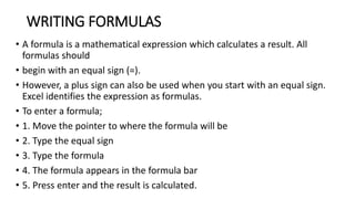
The document provides instructions for writing formulas, performing calculations, formatting cells, creating charts, and saving workbooks in Excel spreadsheets. Key steps include: 1) Writing formulas using cell references and operators like =, +, -, /. 2) Performing calculations by selecting cells and typing formulas like =SUM(A1:A5). 3) Formatting cells by changing number formats, fonts, column widths, and adding currency symbols. 4) Creating charts by selecting data and using the Chart Wizard. 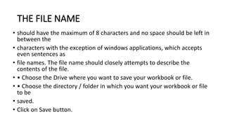5) Saving workbooks by specifying a file name and location.

1. USING SPREADSHEET
MR MUSONDA

2. WRITING FORMULAS
• A formula is a mathematical expression which calculates a result. All
formulas should
• begin with an equal sign (=).
• However, a plus sign can also be used when you start with an equal sign.
Excel identifies the expression as formulas.
• To enter a formula;
• 1. Move the pointer to where the formula will be
• 2. Type the equal sign
• 3. Type the formula
• 4. The formula appears in the formula bar
• 5. Press enter and the result is calculated.

3. ADDITION USING CELL ADDRESSES
• 1. Enter the values
• 2. Select the cell answer
• 3. Type the cell formula
• 4. Enter your responding cells e.g =A1+ A2+A3+A4+A5+A6+A7+A8
• 5. CLICK THE GREEN TICK or enter key

4. MULTIPLICATION USING CELL ADDRESSES
• 1. Enter the values
• 2. Select the answer
• 3. In the cell answer type the equal (=) sign
• 4. Enter your responding cells e.g. = B1* B2*B3* B4* B*B6
*B7*B8*B9
• 5. PRESS THE ENTER KEY or click on the green tick

5. SUBTRACTION USING THE CELL
• 1. Enter your values
• 2. Select your cell answer
• 3. In cell answer, type = sign
• 4. Enter your responding cell e.g
• = D1- D2
• = G5- G7 or = H5-H6

6. DIVISION USING CELLS
• 1. Enter your values
• 2. Select the cell answer
• 3. Type an equal sign in your cell answer
• 4. Enter the responding cells e.g = E 1/E2
• 5. Click on green tick or press enter

7. ADDITION USING : FUNCTION
• 1. Type the following;
• 2. = sum(B12:B16)

8. COPYING FORMULAS
• Copying formulas is similar to other data in a work sheet. To copy
formula
• 1. Select the formula that you wish to copy
• 2. Pull down the edit menu
• 3. Choose copy
• 4. Move the cursor to the first cell in the area were you would like to
place the copy
• 5. To copy data to another work sheet. Change to work sheet.
• 6. Pull down the edit menu
• 7. Choose paste and the data is copied

9. USING RELATIVE AND ABSOLUTE CELL
ADDRESSING
• 1. When you copy a formula from one place to another in the work
sheet, the cells
• 2. that are referenced in the formula are adjusted to compensate for
the movement.
• An absolute reference is a cell reference in a formula that does not
change when copied to a new formula copied.
• 3. To create an absolute reference formula you need only to put s in
front of the address.

10. USING BUILD –IN FUNCTIONS
• Functions help to simplify complex formulas. They are built –in
formulas provided by excel.
• For example, instead of typing =B1+B2+B3+B4+B5+B6 TO Add five
numbers.
• You can use auto sum function from the standard Toolbar.

11. TO USE AUTO SUM
• 1. select the cell to hold the sum
• 2. click on the Auto sum tool from the standard toolbar
• 3. If you need to adjust the range of cells that auto sum has selected,
edit the section
• 4. When the range is corrected, Click on the enter box in the formula
bar or press enter and the total for the range selected is calculated.

12. ADD OR REMOVE A CURRENCY SYMBOL
• 1. Select the cells you want to format
• 2. On the format menu click cells and then click the number tab
• 3. In the category list, Click Currency.
• 4. In the symbol list, do one of the following
• 5. To add currency symbol select the one you want
• 6. To remove currency symbol click none
• Notes: To quickly add the default currency symbol, select the cells you
want to Format and then click currency style on the formatting toolbar

13. TO QUICKLY INSERT CURRENCY SYMBOL
• You can use number formulas to change the appearance of numbers
including dates and times without changing the number behind the
appearance.

14. CHANGING COLUMN WIDTH AND ROW
HEIGHT
• To use the mouse to change row height or width
• 1. Move the pointer to the heading for the row or column
• 2. Move to the column or border
• 3. Drag the border to its new location.
• 4. Release the mouse button and the border is reset.
• To reset the width for the best fit, double-click on the top right edge
of the column

15. CREATING CHARTS
• A chart can be created as part of the worksheet or as a separate file. A
Chart that is created as part of a worksheet embedded chart.
• To create the chart as a separate file.
• 1. Enter summary report
• 2. Select them all
• 3. Click on chart wizard icon
• 4. Click on next two times
• 5. Click on chart title and type your [weeklybudget]
• 6. Click on category x [items]
• 7. Click on value y[kwacha]
• 8. Click on finish.

16. HOW TO MOVE THE CHART
• 1. select your chart
• 2. drag it on the middle

17. HOW TO RESIZE THE CHART
• 1. select your chart
• 2. retrieve double headed arrow
• 3. drag to your required sizes

18. HOW TO CHANGE A BAR CHART TO PIE
CHART
• 1. select your chart
• 2. click on the chart icon arrow down
• 3. click on pie chart/line chart

19. CHANGE CATEGORY AXIS LABELS
• to change category axis label on the work sheet, click the cell that
contains the label name: change the type new name, and then press
ENTER
• to change category axis label on the chart and then click on the chart

20. CHANGE DATA SERIES NAMES LEGEND TEXT
• • to change legend text or data series names on the worksheet ,click the
cell that contains the data series name you want to change, type the new
name , and then press enter
• To change legend text or data series names on the chart,
• click the chart and then

21. CON…
• click source data on the chart menu. On the series tab, click the data
series names you want to change.
• In the name box, specify the worksheet cell you want to use as the
legend text or data series name.
• You can also type the name you want to use.
• If you type a name in the name box the legend text or data series
name is no longer linked to a worksheet cell.
• Note: This procedure does not apply to pivot chart reports. How to
rename a field or item in a pivot chart report.

22. CHANGE DATA LABELS
• To change data labels on the worksheet, click the cell that contains the
information
• you want to change, type the new text or value, and then press ENTER.
• - To change data labels on the chart, click once on the data label you
want to change
• to select the data labels for the entire series, and then click again to
select the individual
• data label. Type the new text or value, and then press ENTER
• If you change the data label text on the chart, it is no longer linked to a
worksheet cell.

23. NOTE
• Note: you cannot change data labels on the worksheet for a pivot
chart report.
• You can however, change individual data labels on a pivot report.
• Changes to data labels are retained pivot chart reports.
• When you subsequently change the view of the chart or its associated
pivot table report.
• Before you modify data labels or other formatting in a Pivot chart
report make sure you are satisfied with the layout.

24. EDIT CHART AND AXIS TITLE
• 1. Click the title you want to change.
• 2. Type the new text you want.
• 3. Press ENTER change the cell range used to create a chart
• 4. Click the chart you want to change.
• 5. On the chart menu click source data and then click the data range
tab

25. CON…
• 6. Make sure the entire reference in the data range box is selected.
• 7. On the worksheet select the cells that contain the data you want to
appear in the
• chart.
• 8. If you want the column and the row labels to appear in the chart
include the cells
• that contain them in the selected range values in a chart

26. CON…
• This procedure does not apply to pivot chart reports learn about
using different source
• data for pivot chart e.g. range value in a chart.
• The values in a chart are linked to the worksheet from which the
chart is created.
• The chart is updated when you rearrange values in a chart.
• The values in a chart are linked to the worksheet from which the
chart is created.
• The chart is updated when you change data on the worksheet.

27. CON…
• Open the worksheet that contains the plotted chart.
• In the cell that contains the value you want to change type a new
value.
• Press ENTER
• Note: This procedure does not apply to pivot chart report

28. TO PRINT A WORK SHEET
• There are many times when you only want to print a portion of a
work sheet. This is easily done through the print range function.
• TO PRINT
• • Select the area to be printed
• • Click the print area button on the page layout tab
• • Click select print area.

29. SAVING A WORKBOOK
• To save the workbook:
• • Click FILE from the menu bar.
• • Click SAVE AS (the save as dialog box appears).
• • Under File Name enter the name you wish to give to your
workbook.

30. THE FILE NAME
• should have the maximum of 8 characters and no space should be left in
between the
• characters with the exception of windows applications, which accepts
even sentences as
• file names. The file name should closely attempts to describe the
contents of the file.
• • Choose the Drive where you want to save your workbook or file.
• • Choose the directory / folder in which you want your workbook or file
to be
• saved.
• Click on Save button.