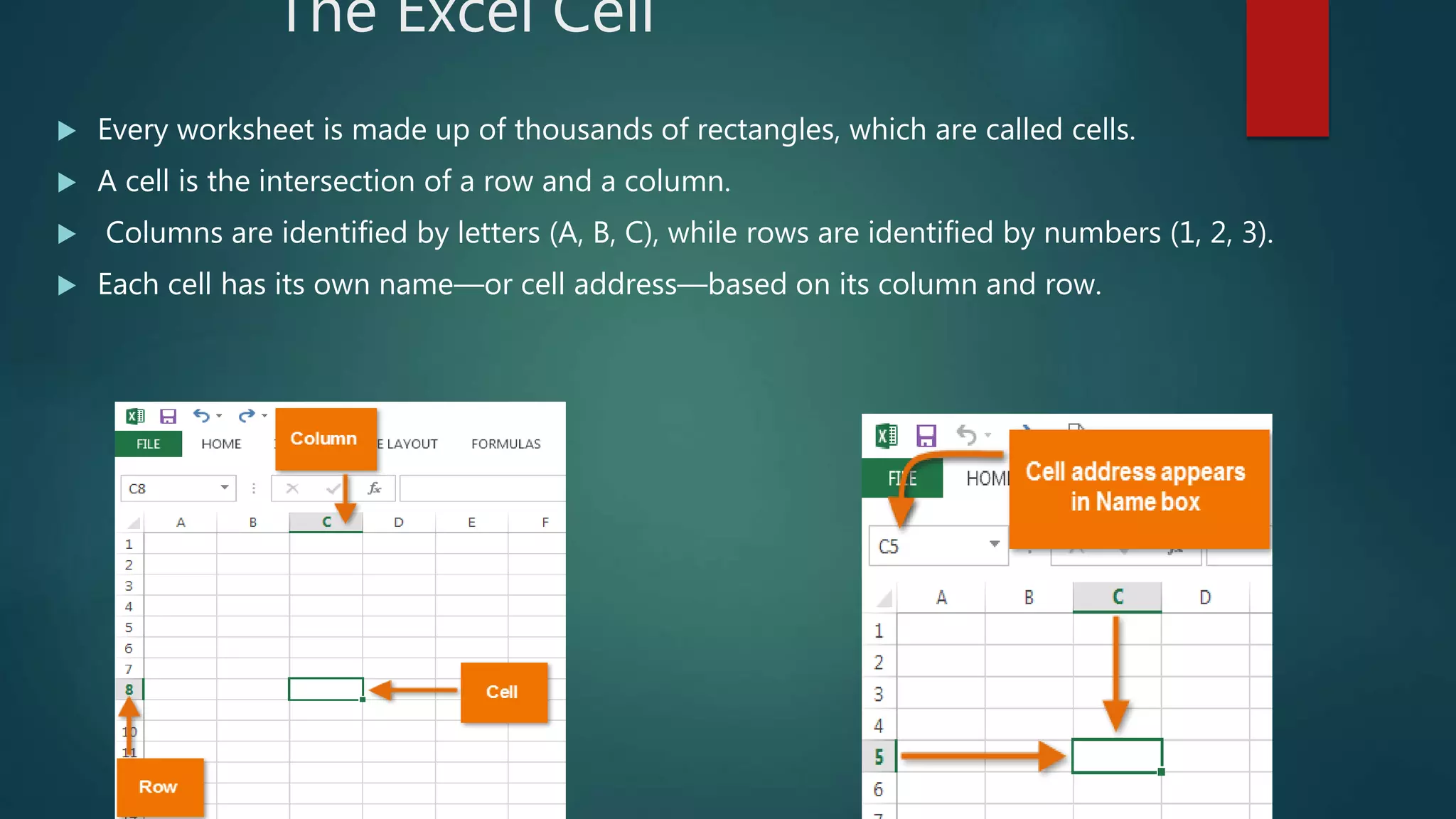
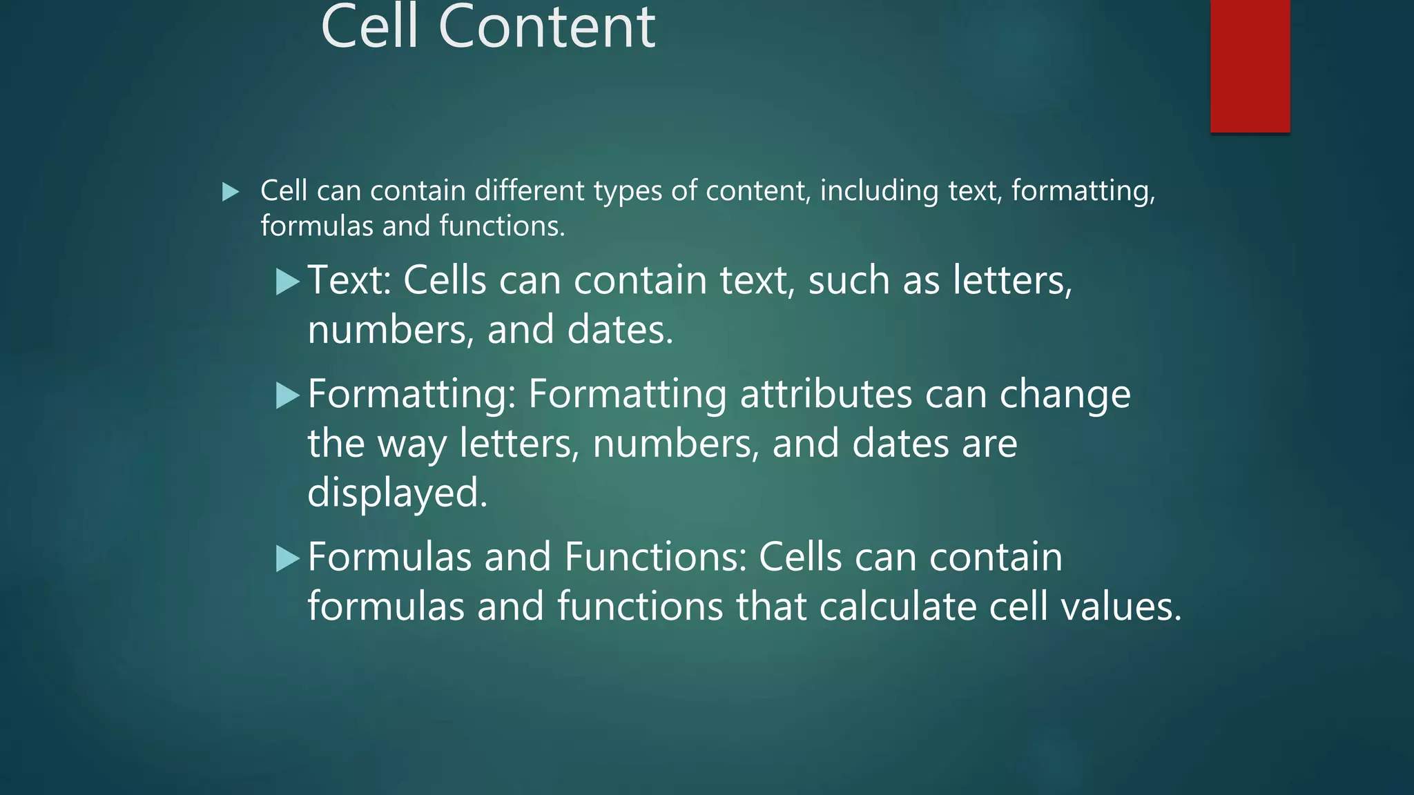
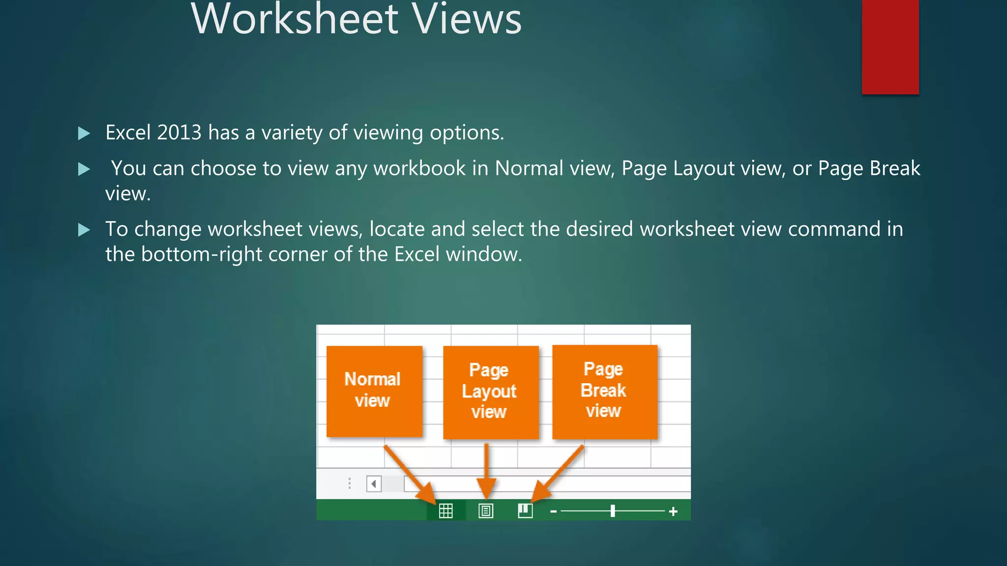
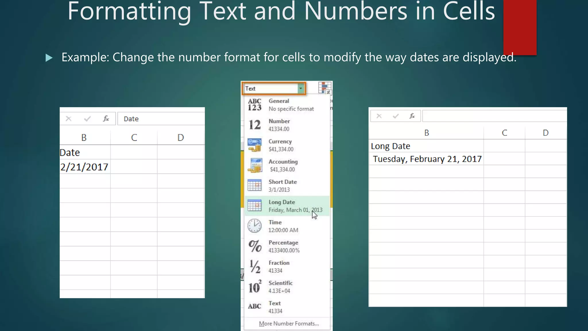
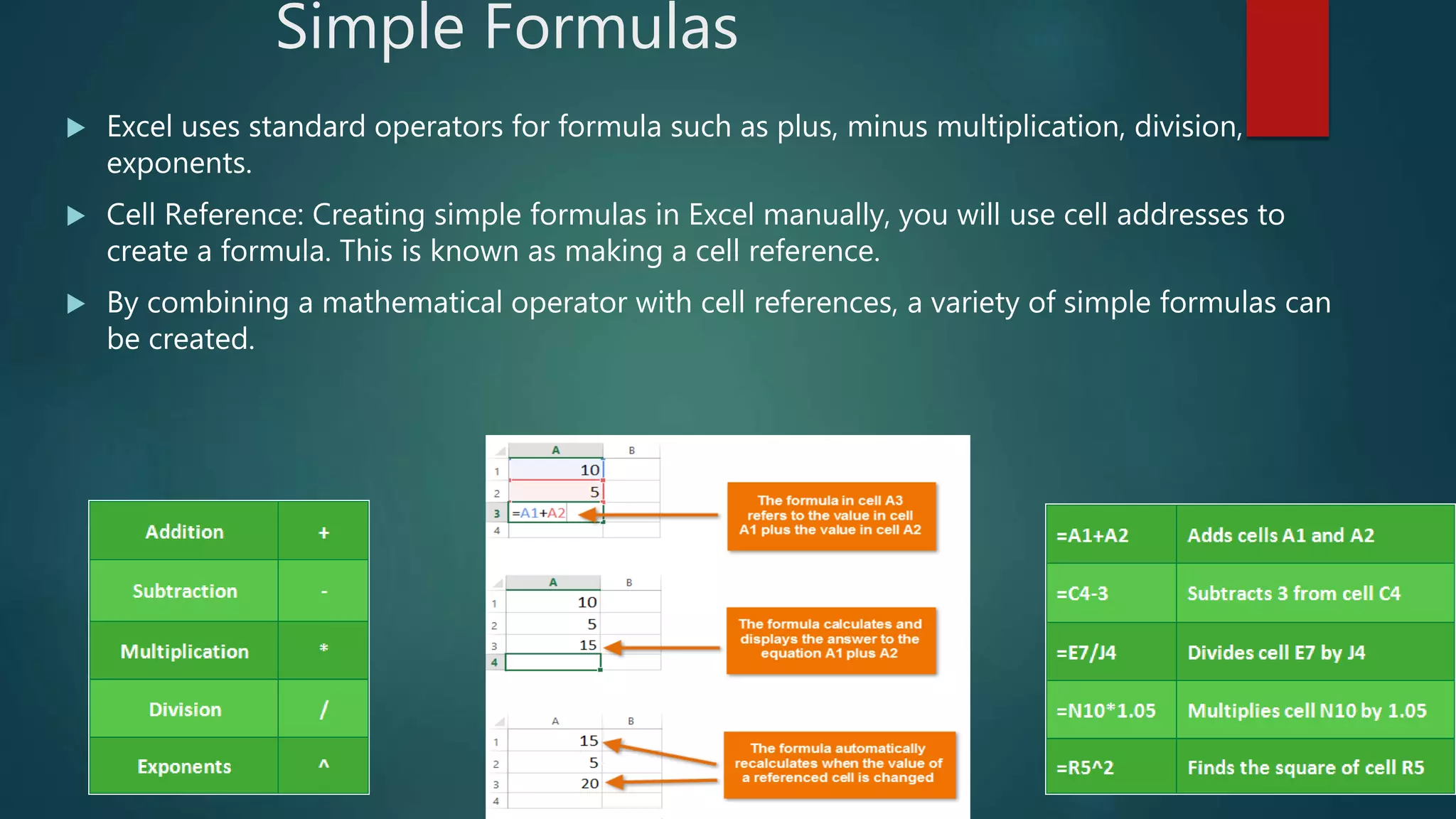
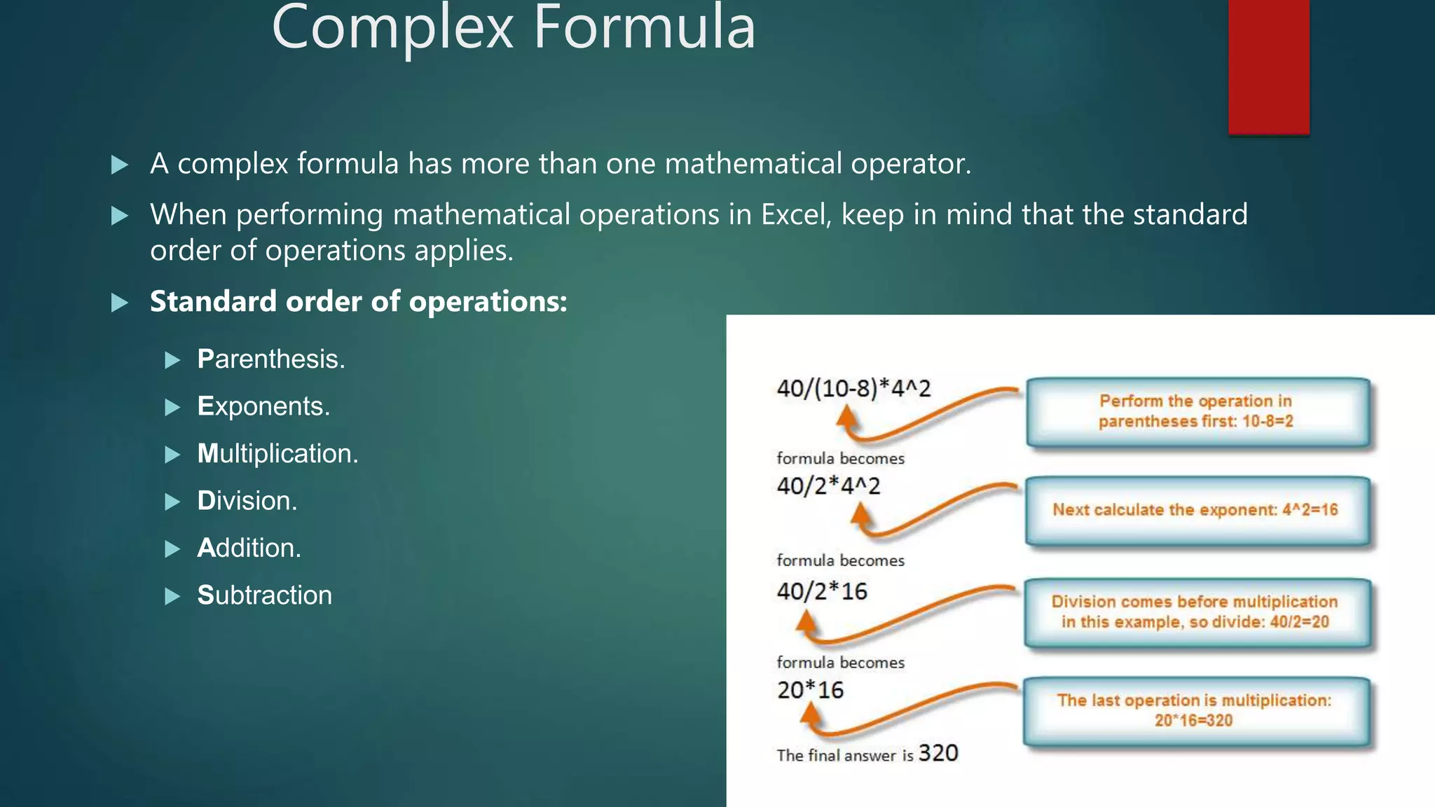
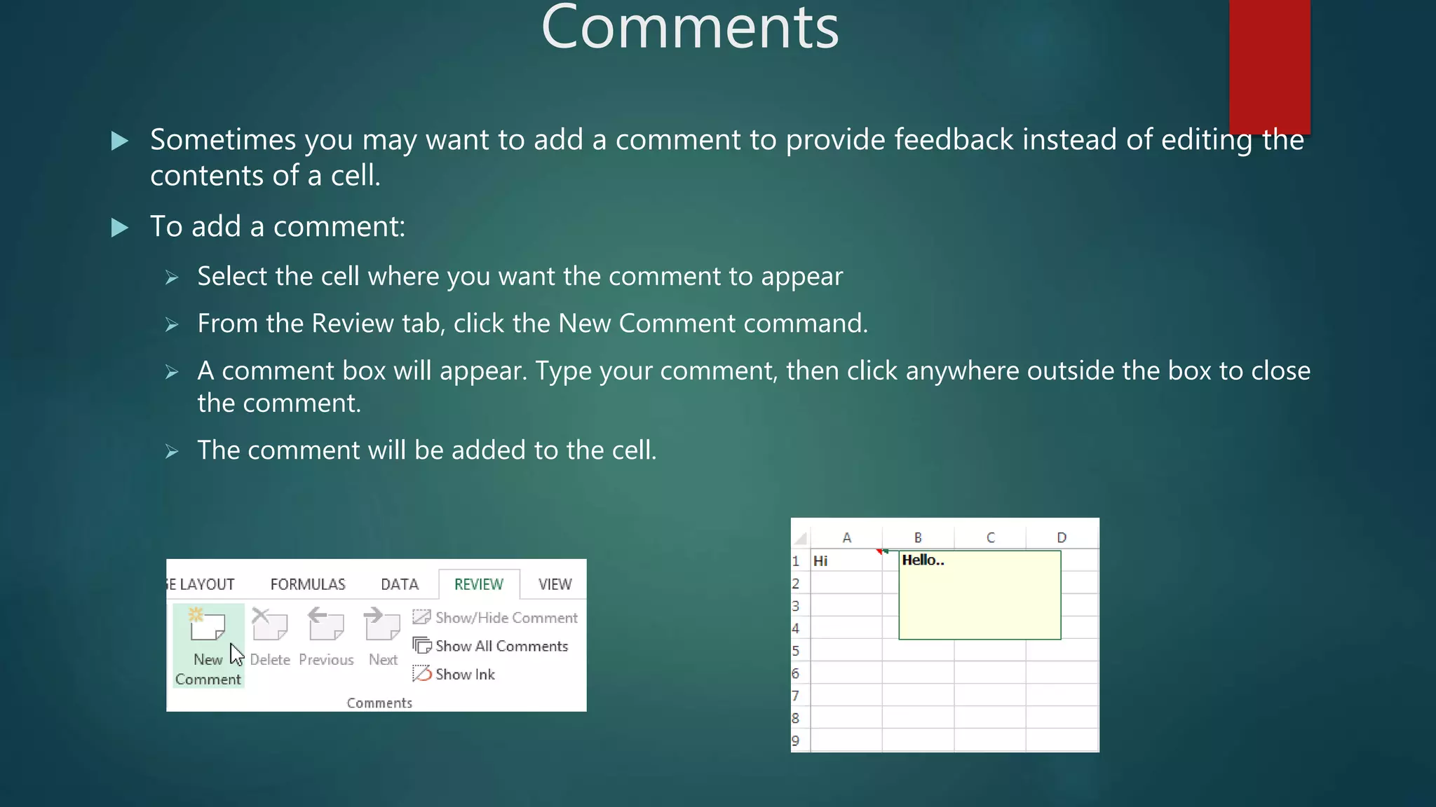
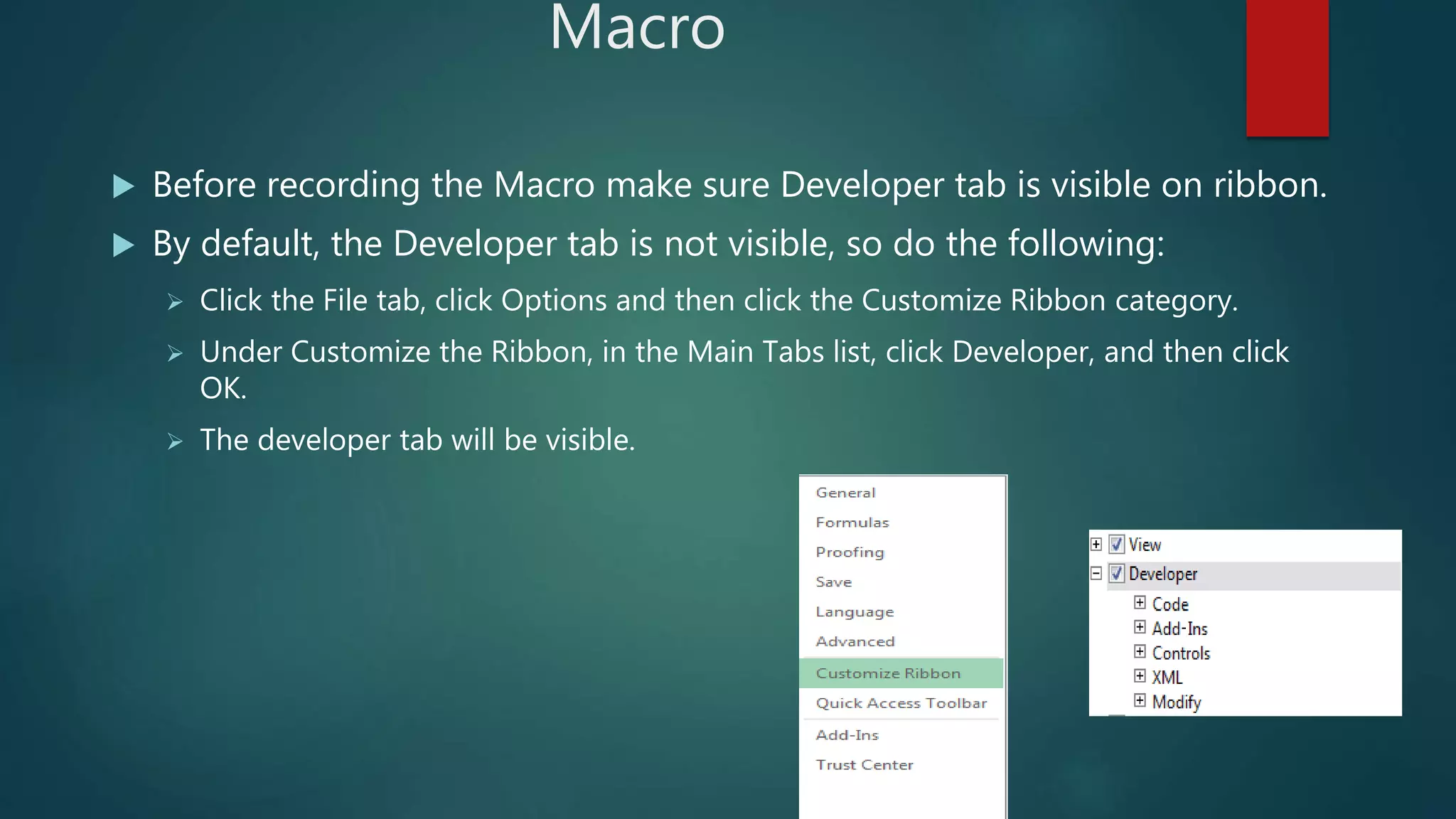
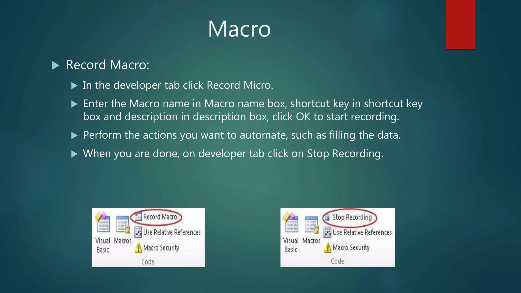
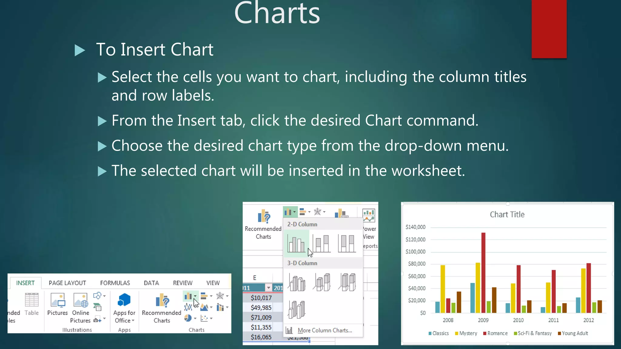
Excel 2013 is a spreadsheet program that allows users to store, organize, and analyze data. It features tools like formulas, functions, charts and pivot tables. In Excel, data is organized into cells within a worksheet. Cells can contain text, numbers, formulas or other content. Worksheets can be viewed and formatted in different layout views. Formatting options and functions allow for analysis of data through calculations and visualization. Pivot tables and charts provide interactive summaries and visual representations of worksheet data. Macros allow repetitive tasks to be automated. Advanced features include comments, filtering, sorting, tables and other analysis tools.