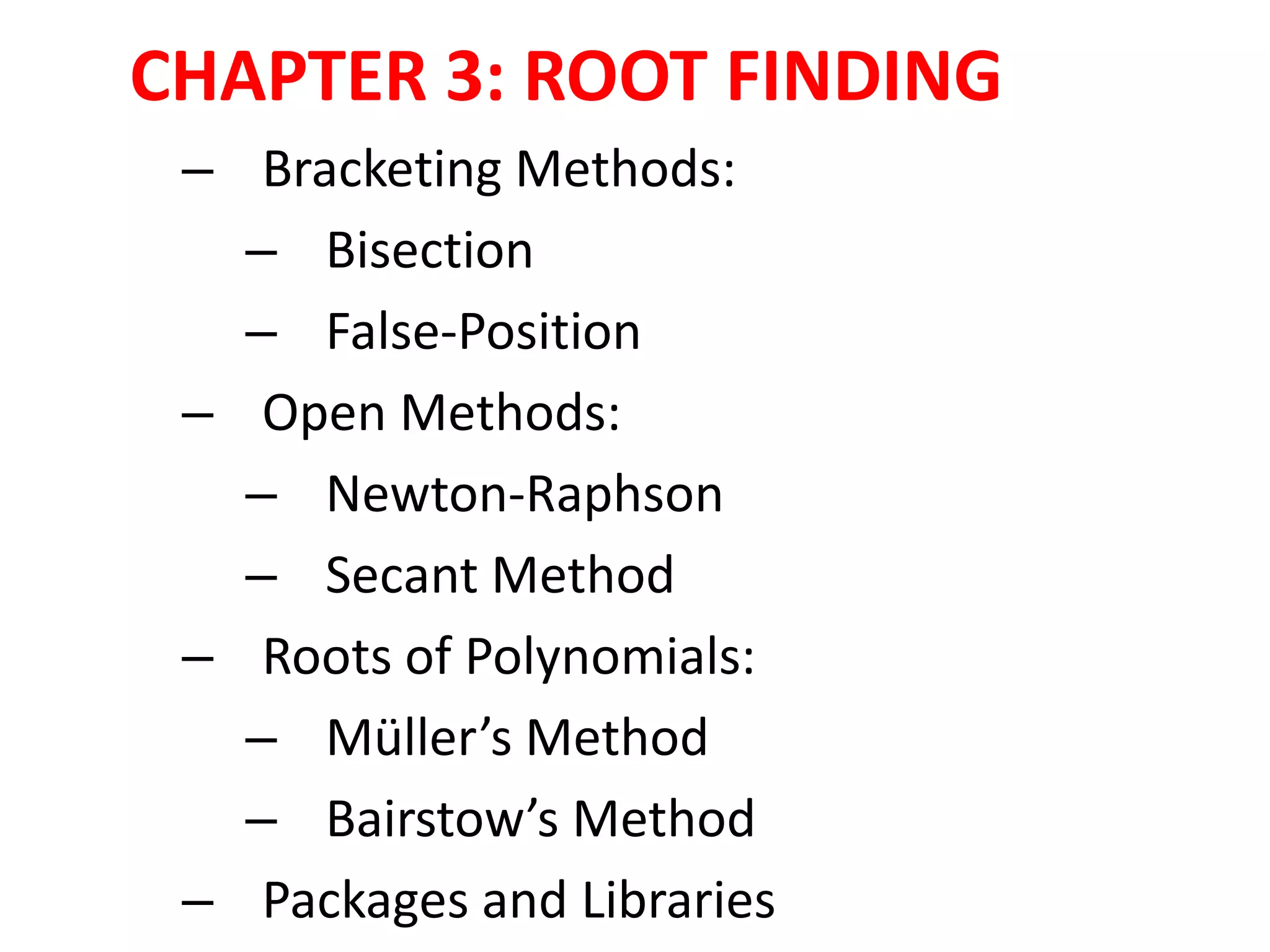
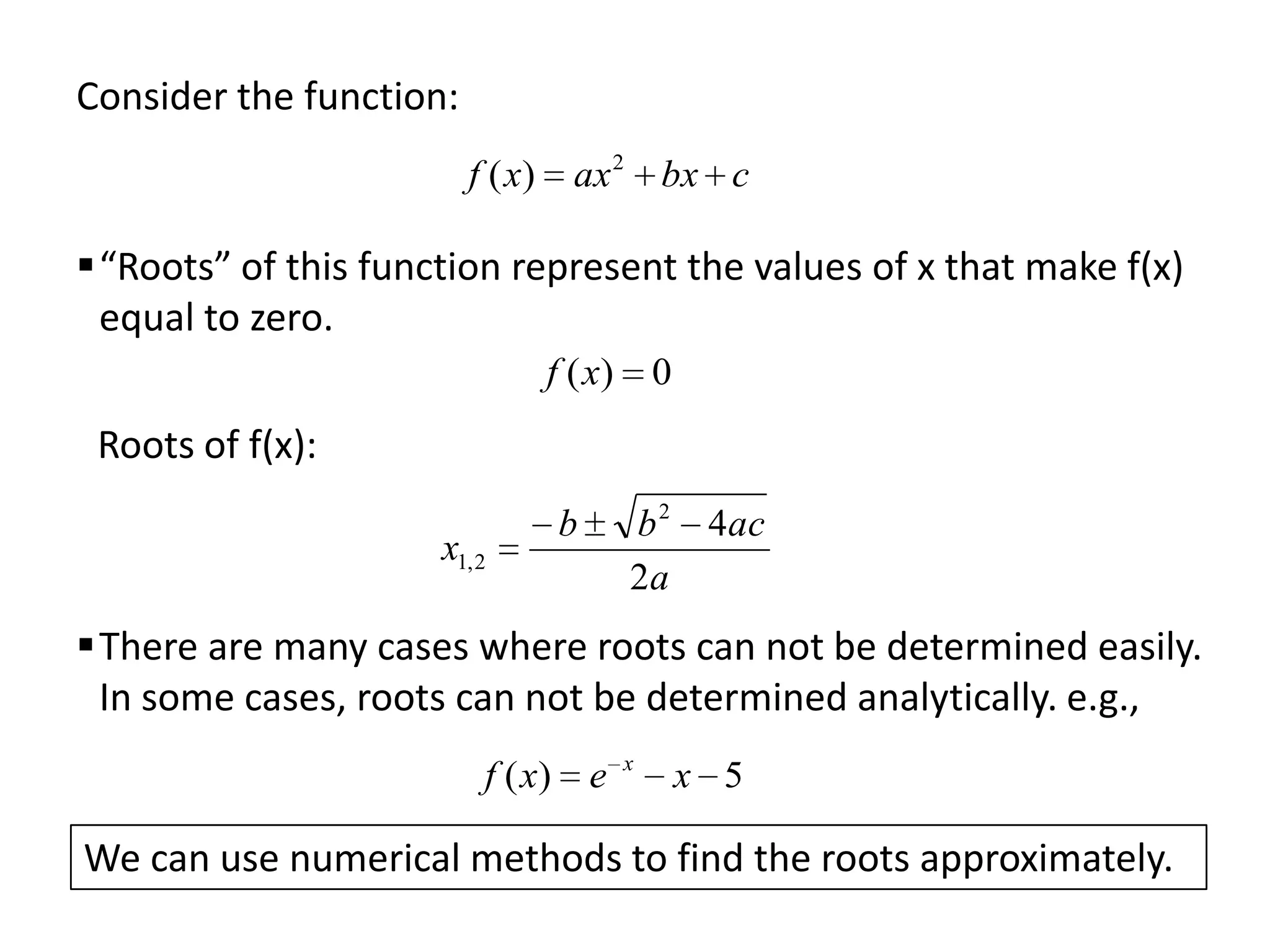
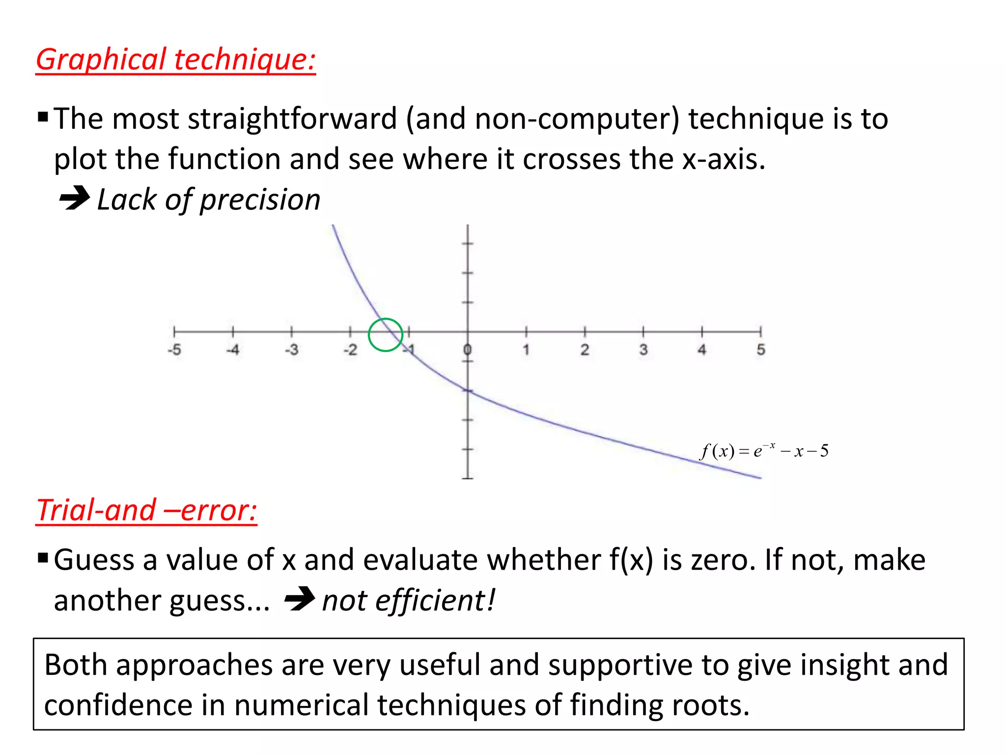
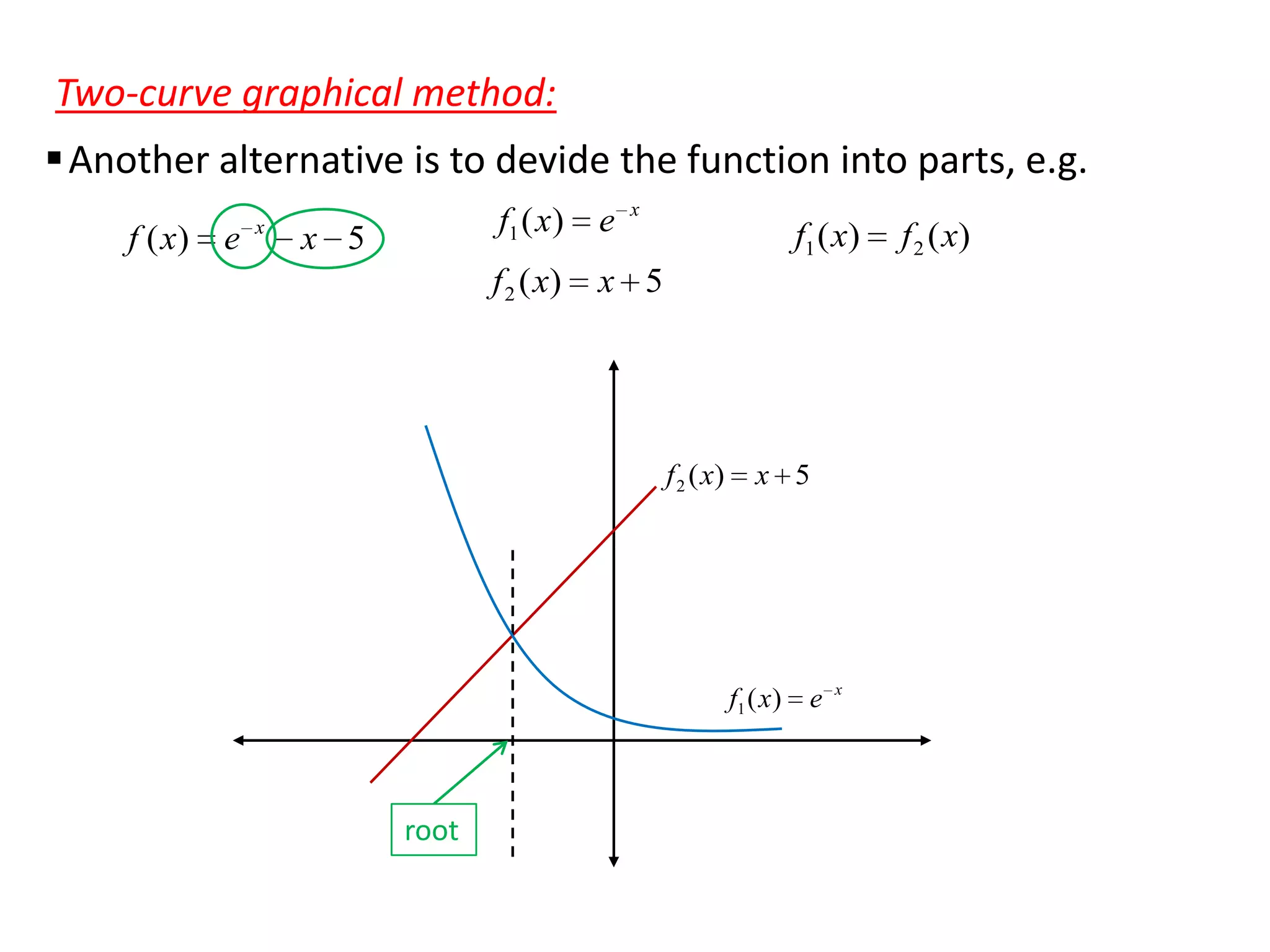
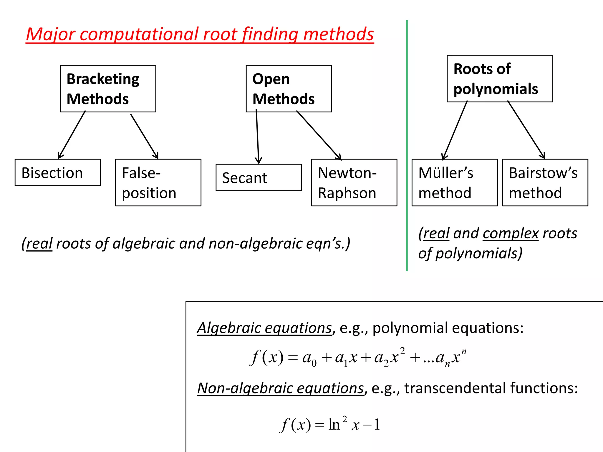
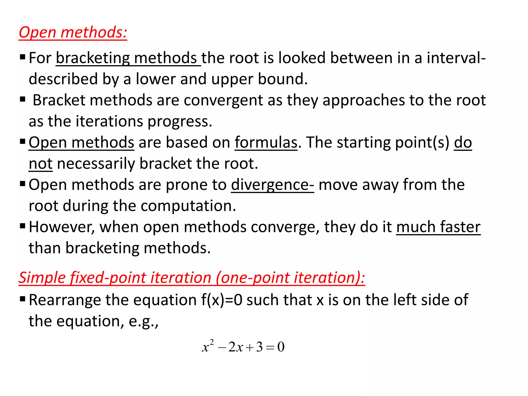
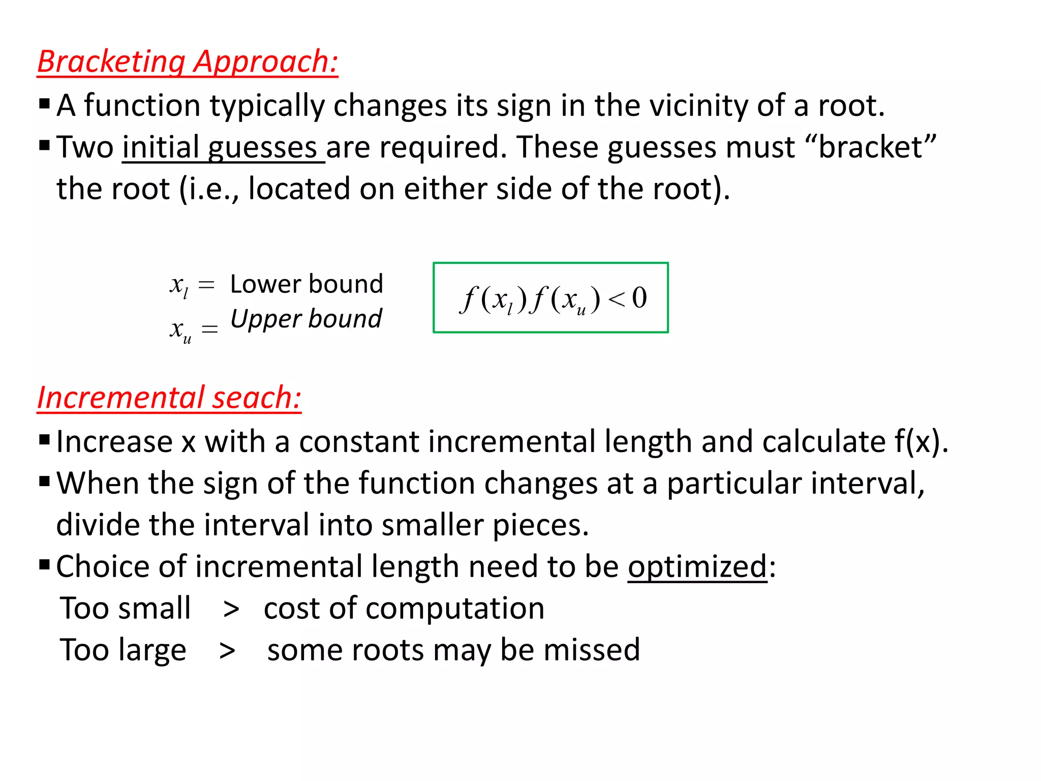
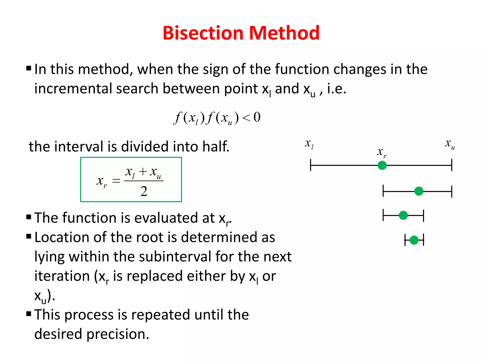
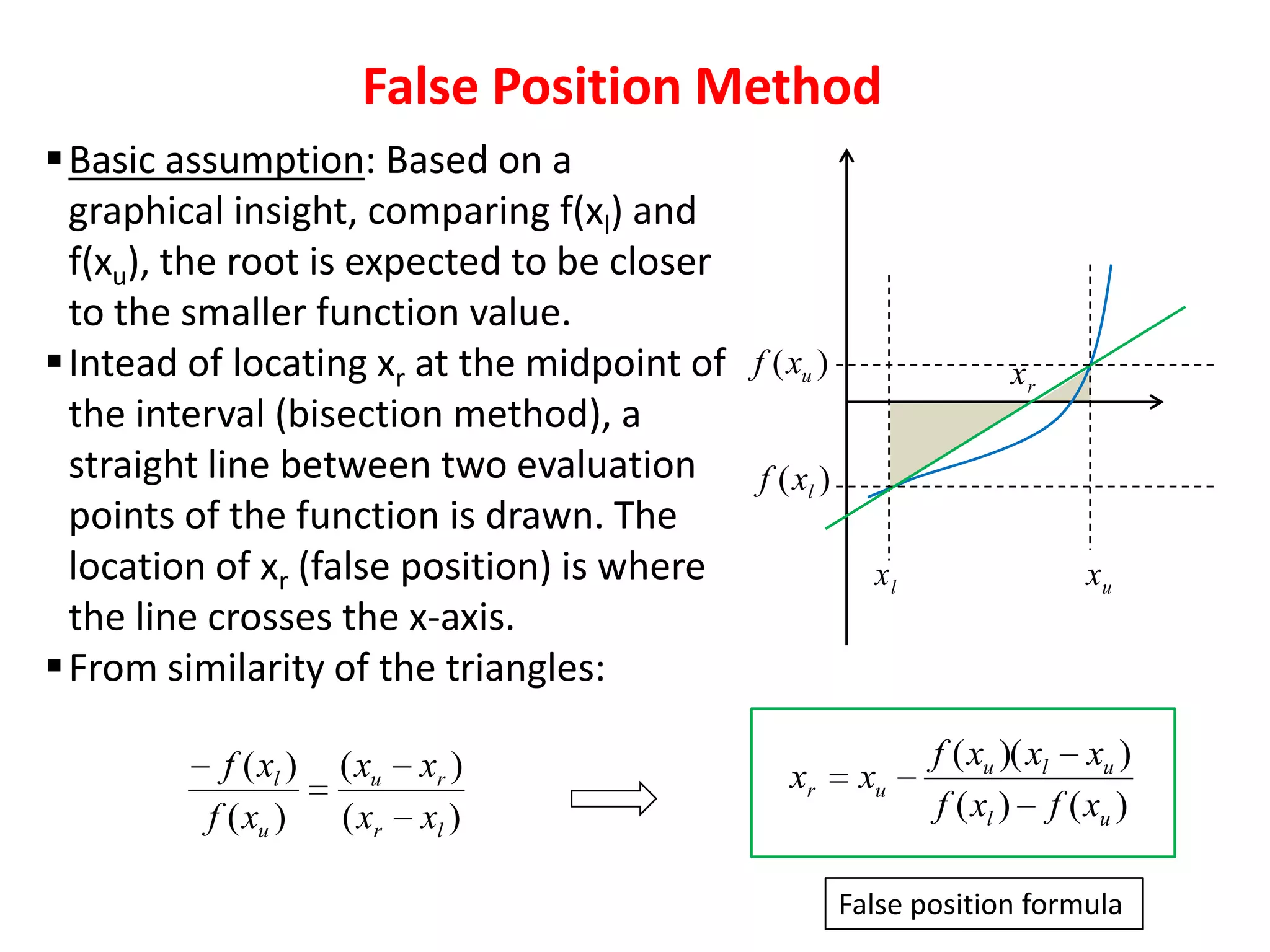
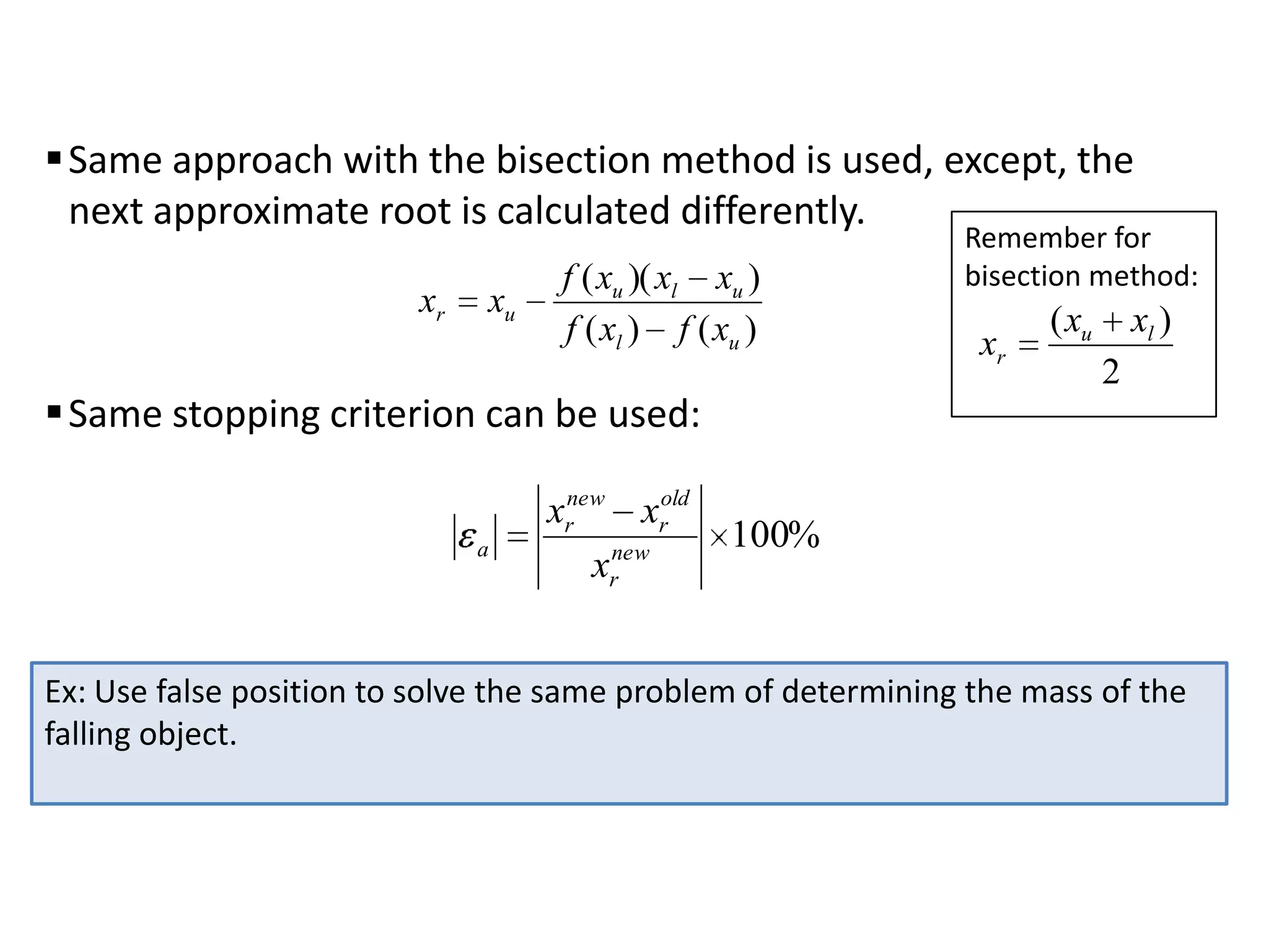
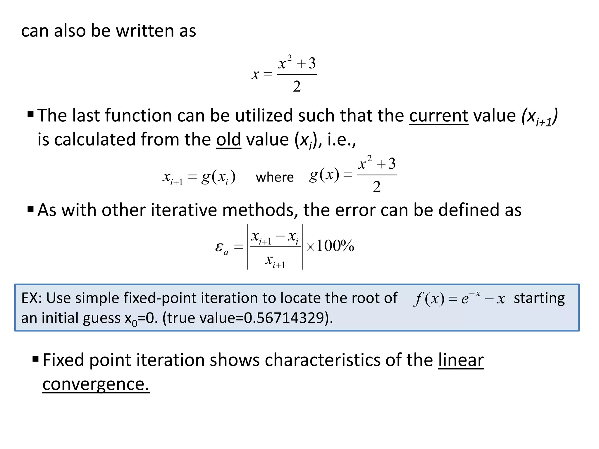
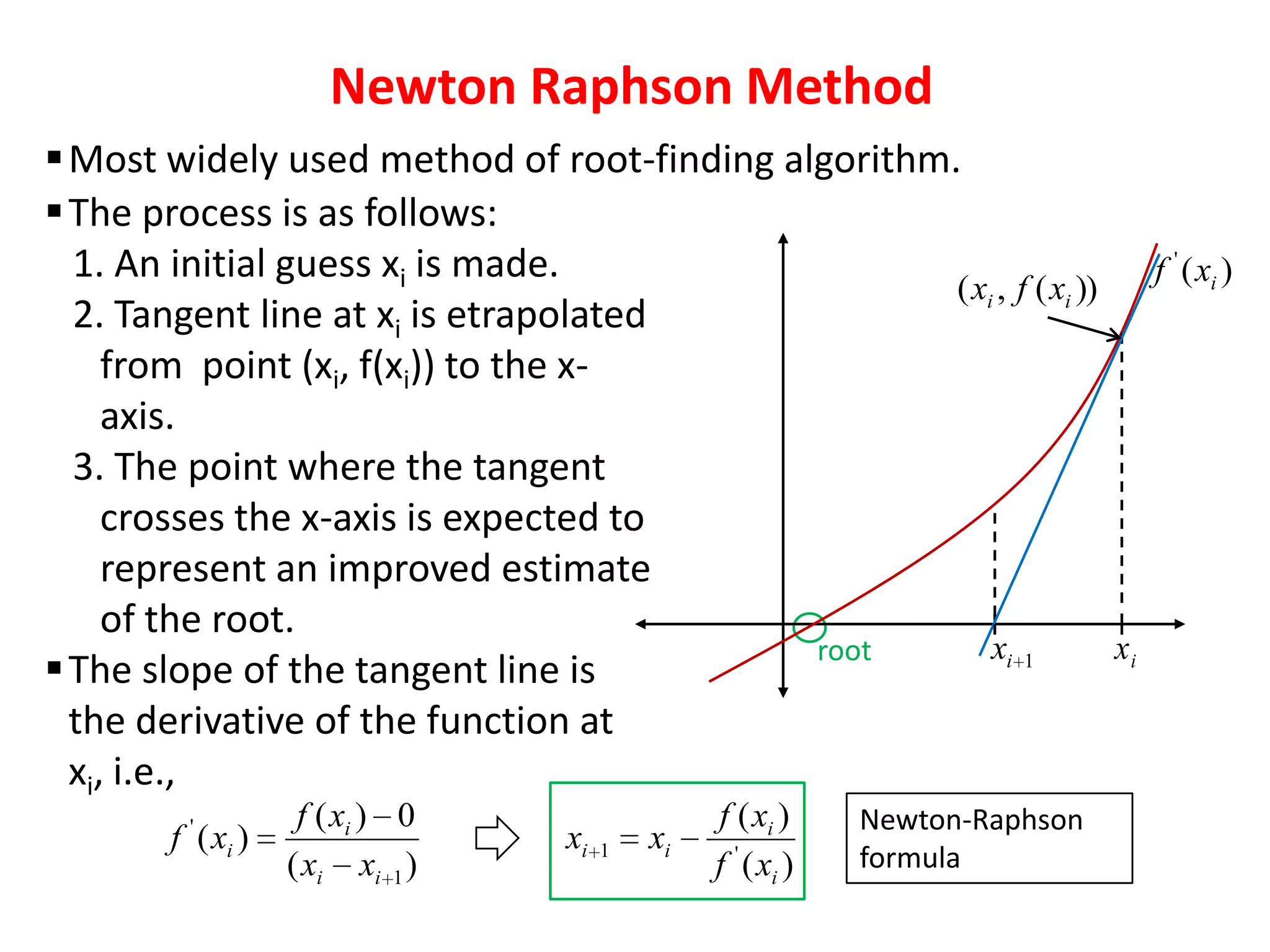
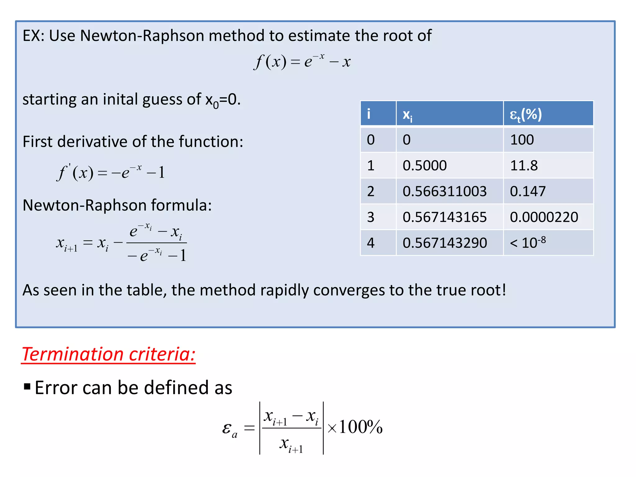
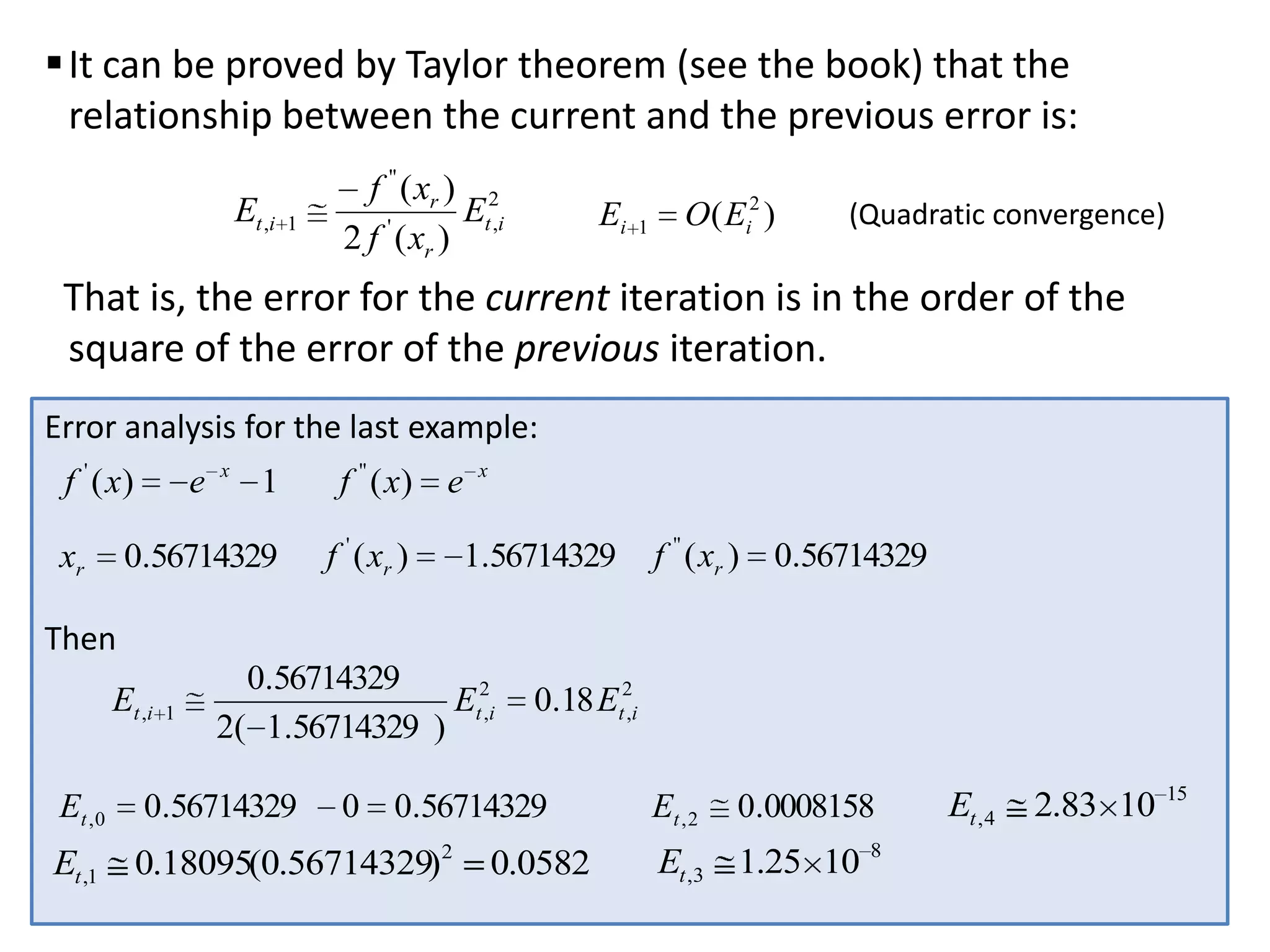
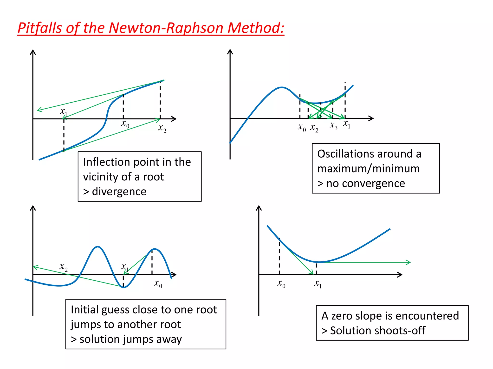
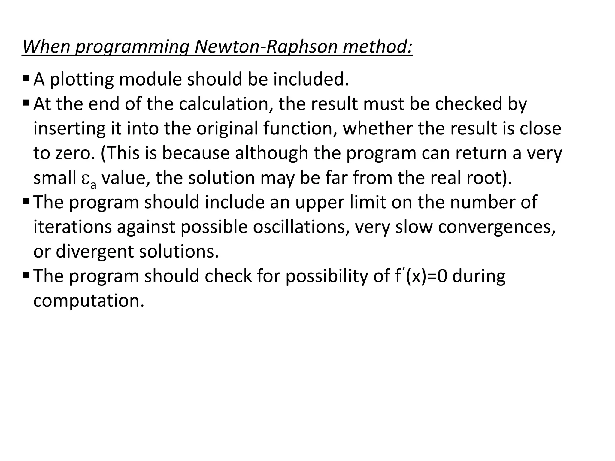
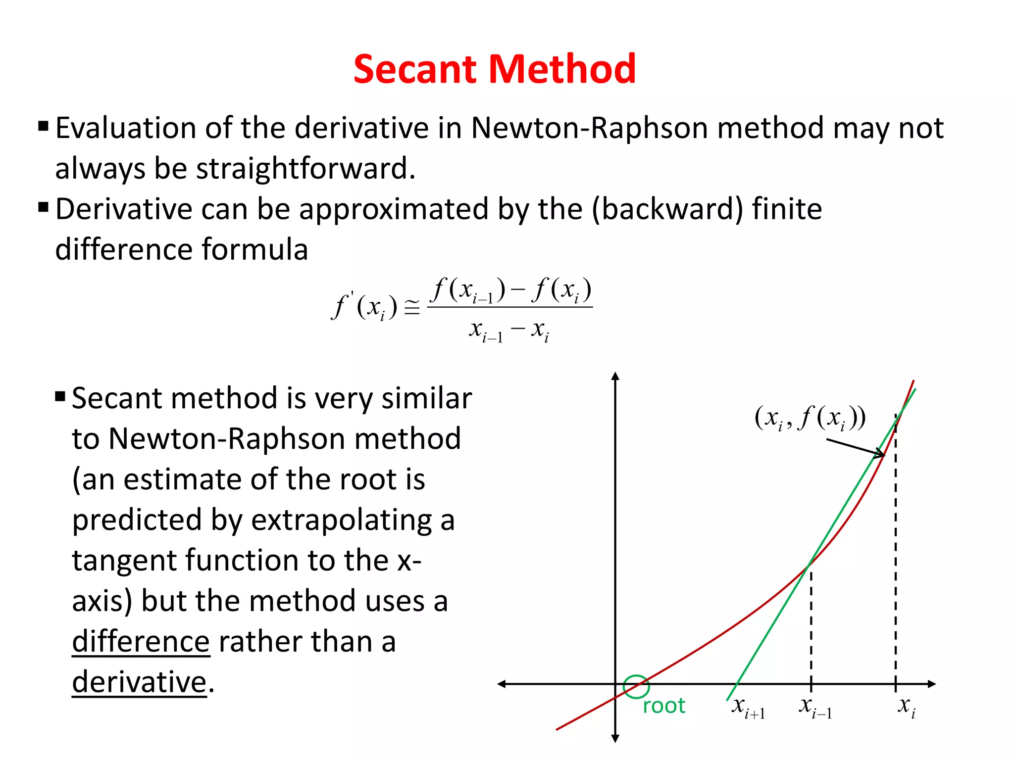
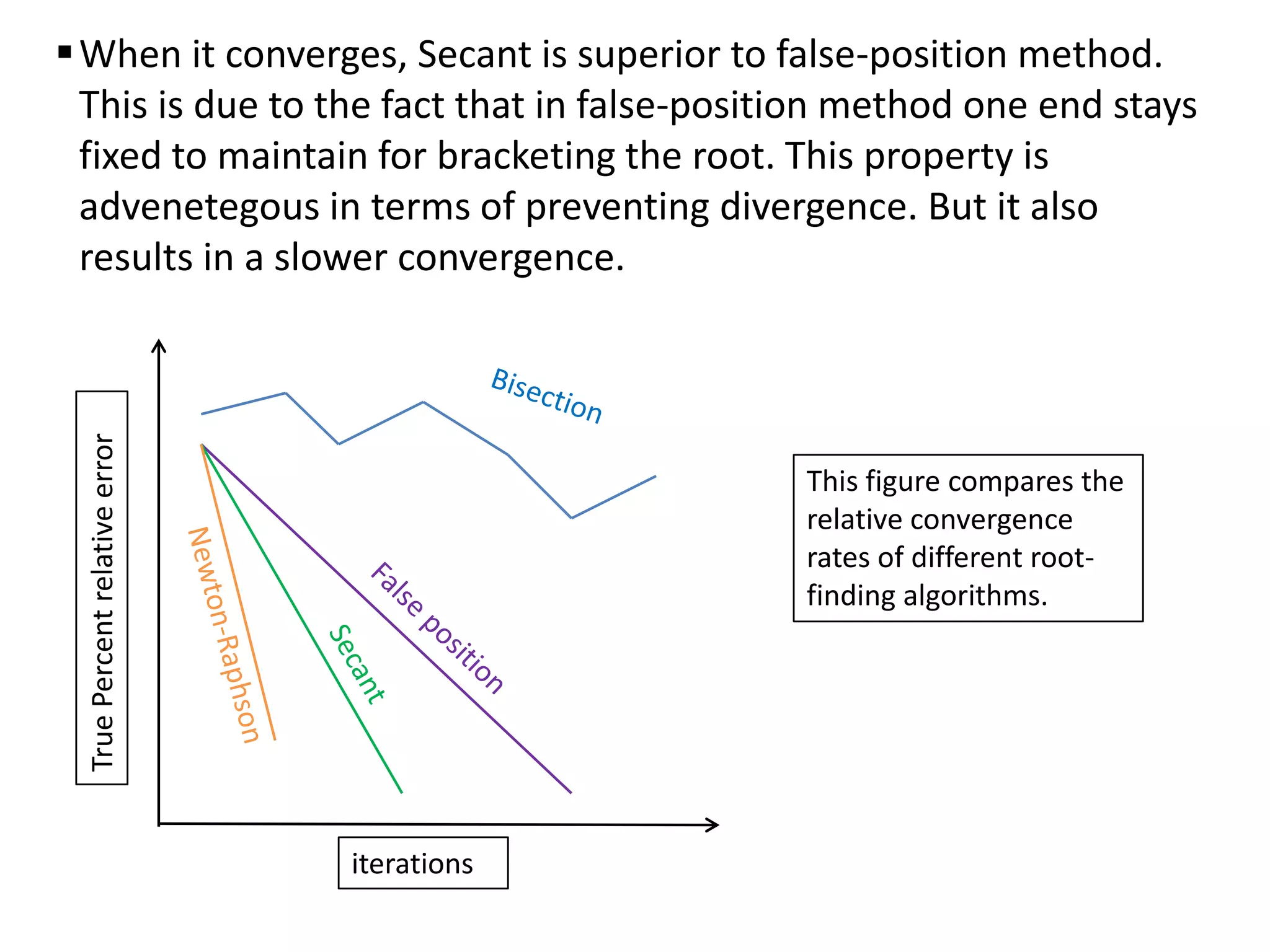
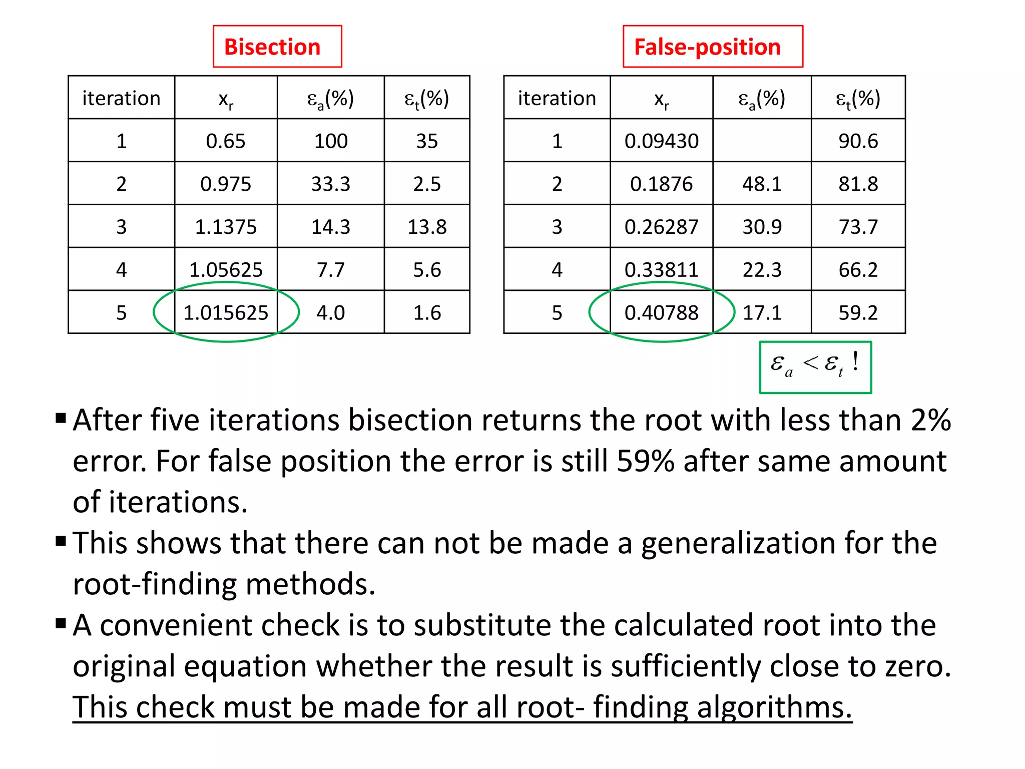
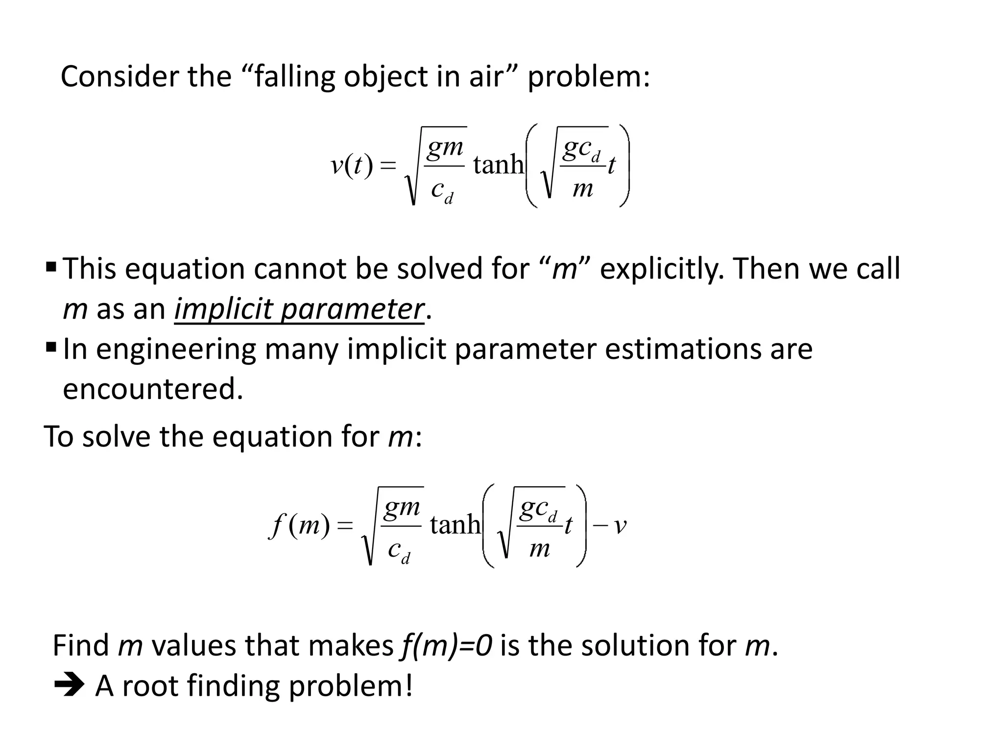
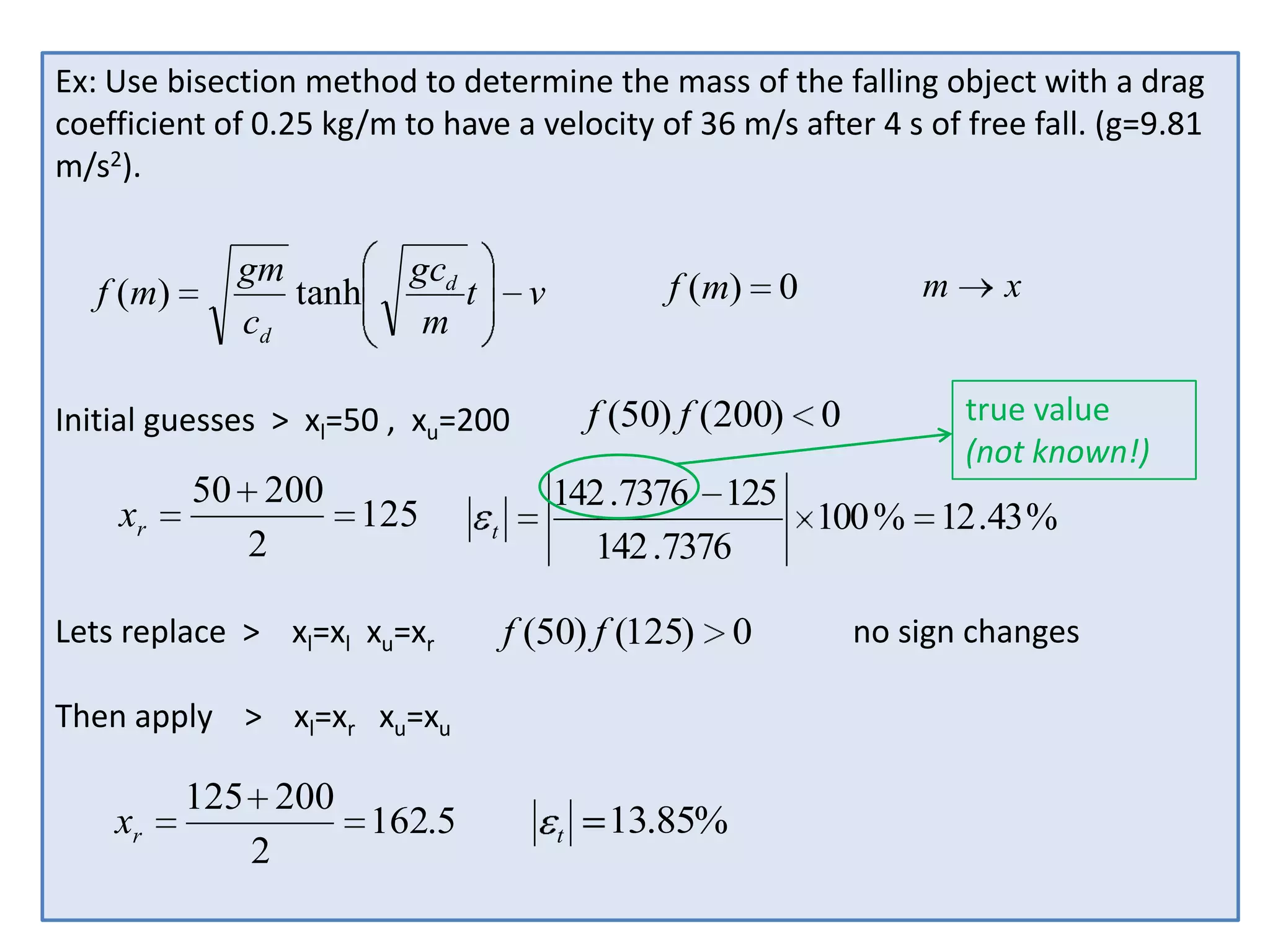
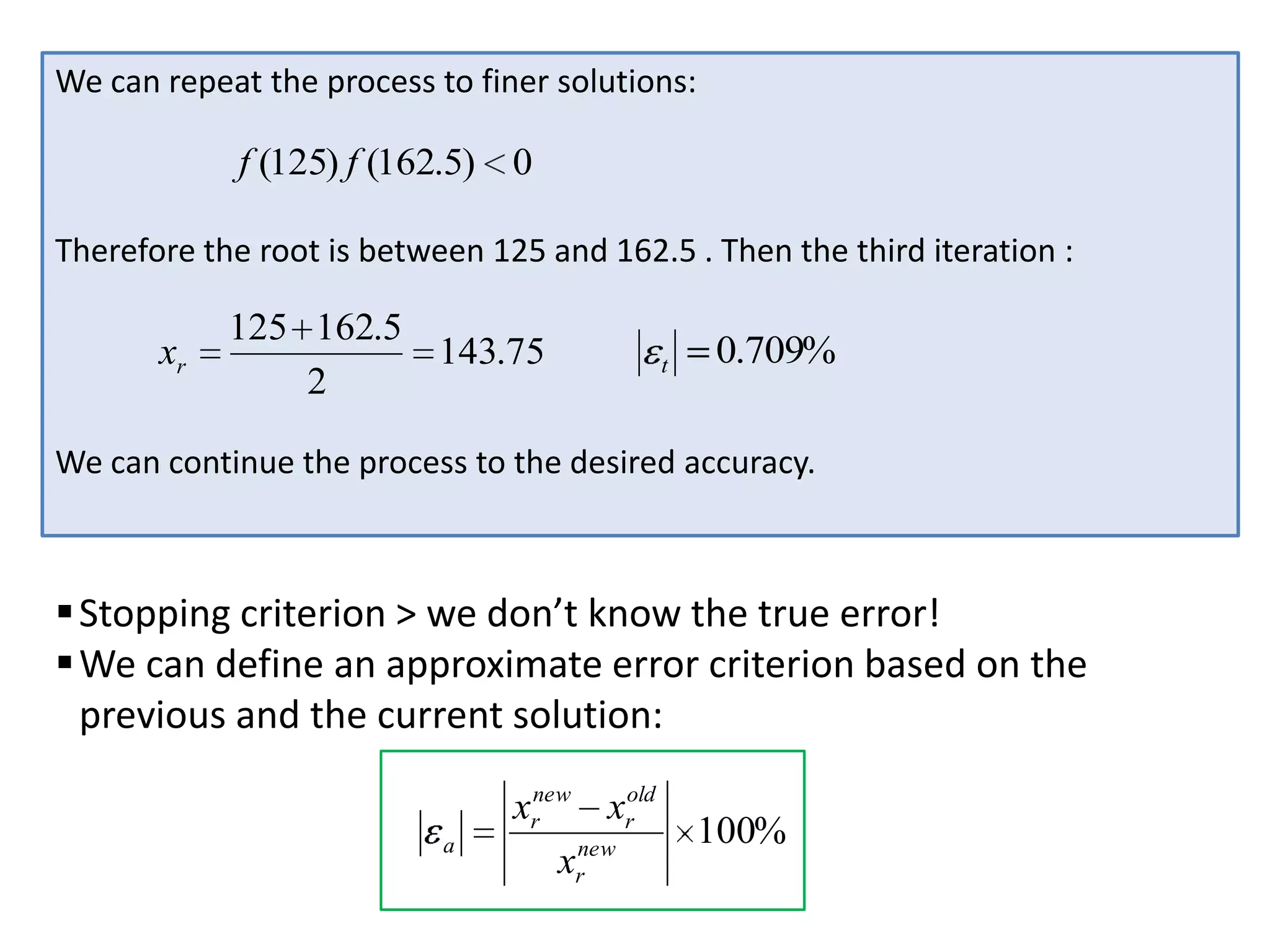
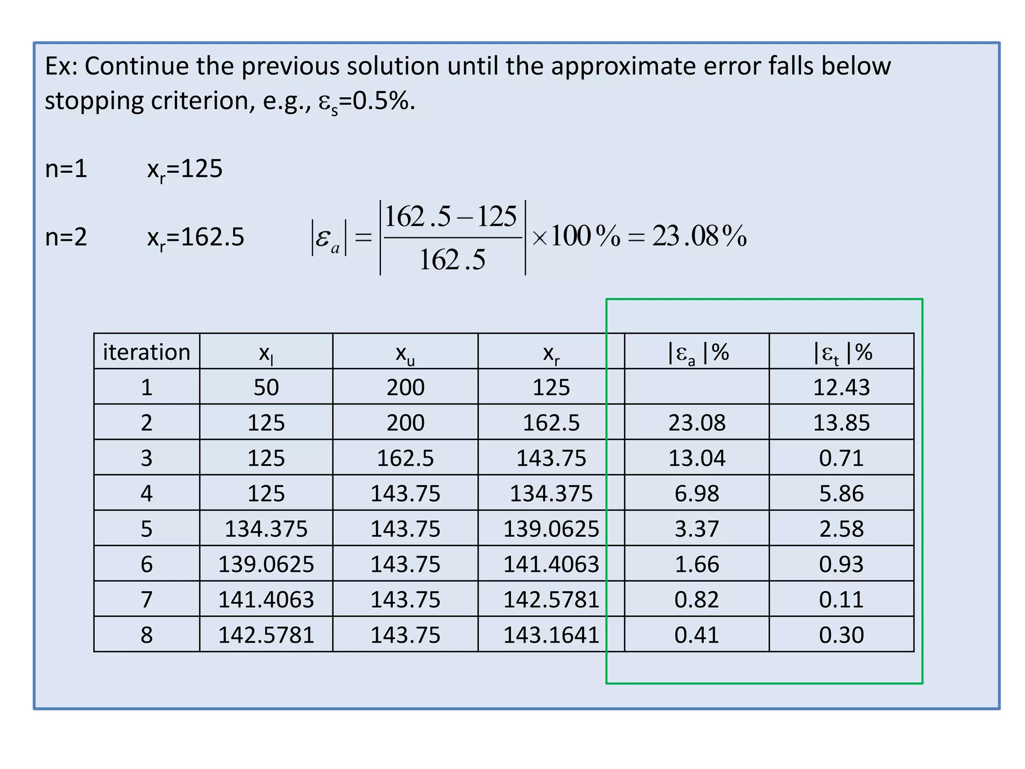
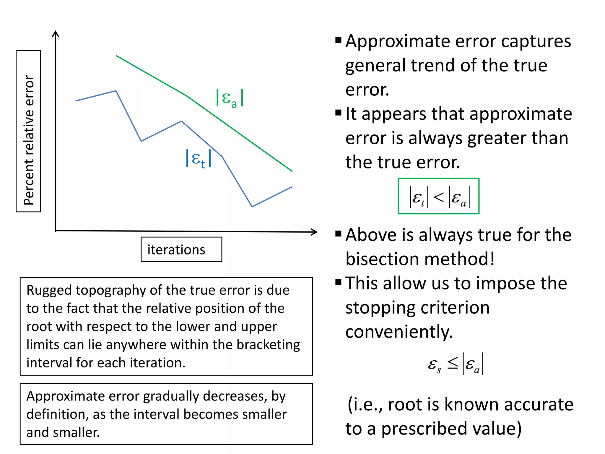
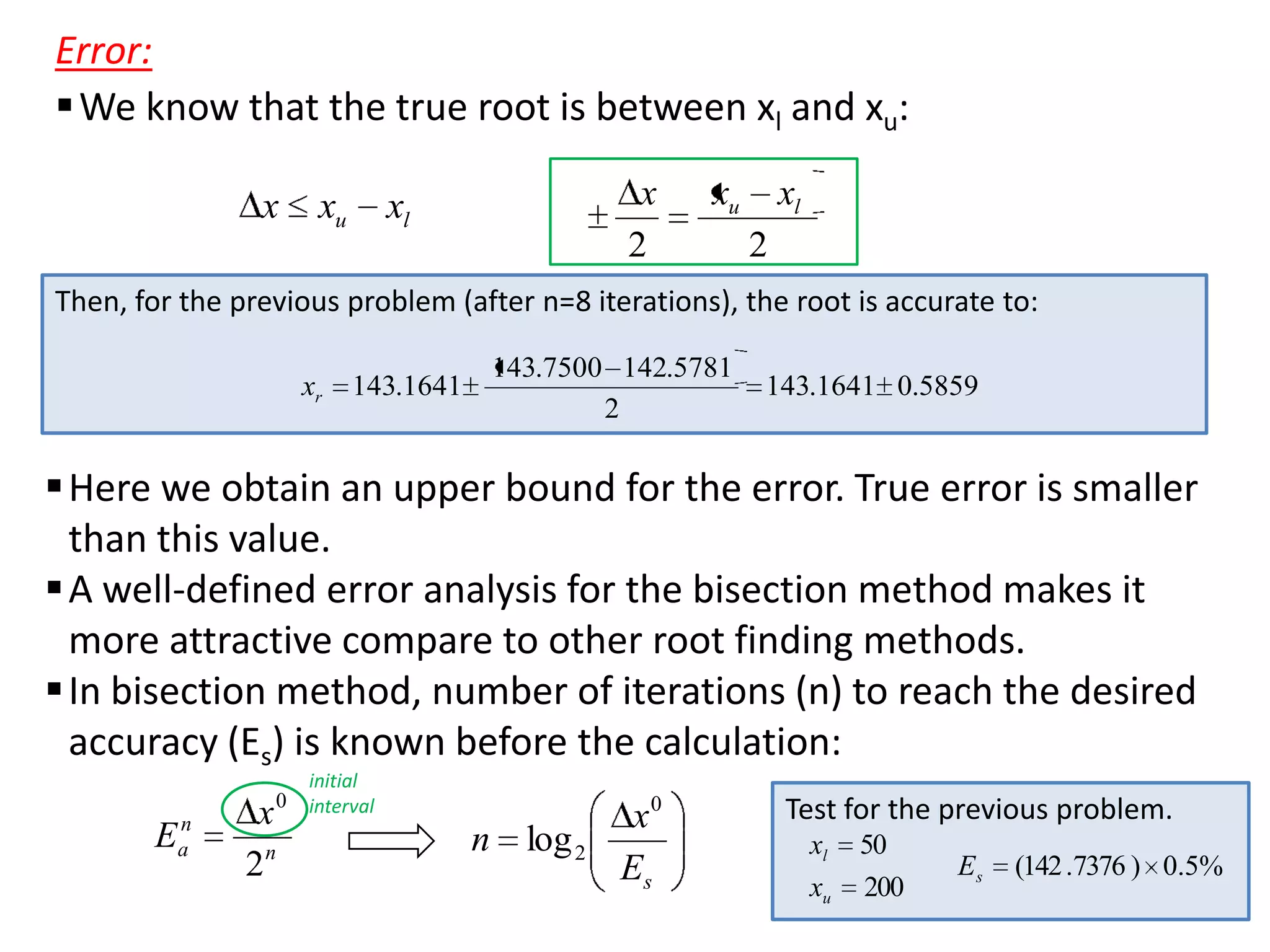
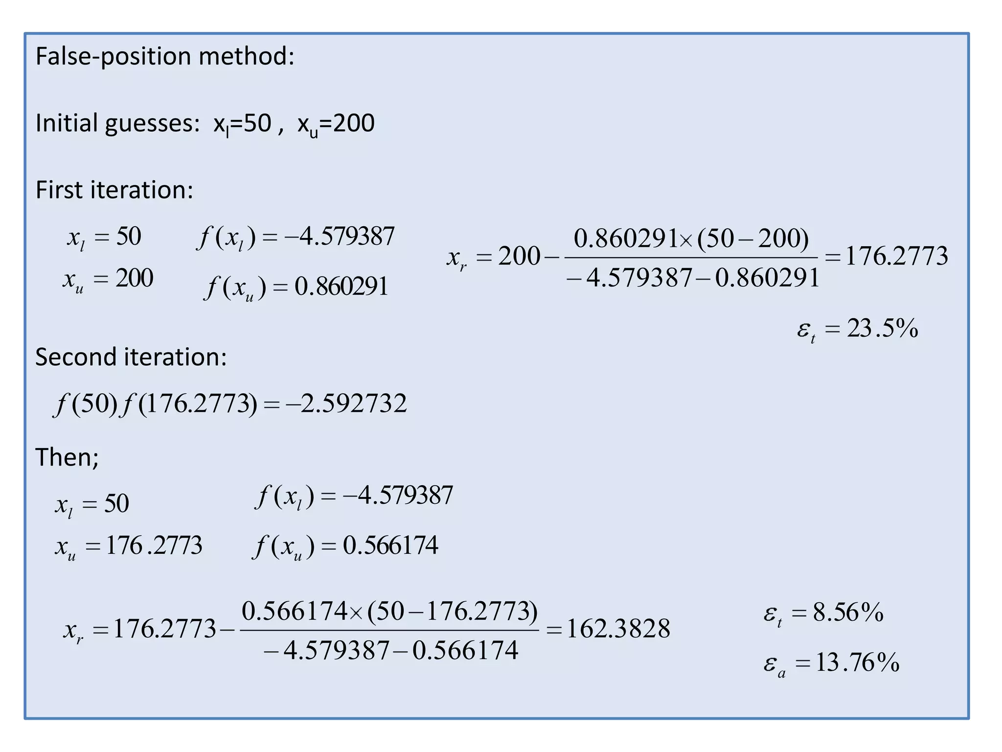
The document discusses various numerical methods for finding roots of functions, including: - Bracketing methods like bisection and false position that search between initial lower and upper bounds. - Open methods like Newton-Raphson and secant that do not require bracketing but may not converge. - Techniques for polynomials like Müller's and Bairstow's methods. Examples demonstrate applying bisection, false position, and Newton-Raphson to find the mass in a falling object problem. The convergence properties and relative performance of the different methods are analyzed.

1. CHAPTER 3: ROOT FINDING
– Bracketing Methods:
– Bisection
– False-Position
– Open Methods:
– Newton-Raphson
– Secant Method
– Roots of Polynomials:
– Müller’s Method
– Bairstow’s Method
– Packages and Libraries

2. Consider the function:
ax 2 bx c
f ( x)
“Roots” of this function represent the values of x that make f(x)
equal to zero.
f (x) 0
Roots of f(x):
x1, 2
b2
2a
b
4ac
There are many cases where roots can not be determined easily.
In some cases, roots can not be determined analytically. e.g.,
f ( x)
e
x
x 5
We can use numerical methods to find the roots approximately.

3. Graphical technique:
The most straightforward (and non-computer) technique is to
plot the function and see where it crosses the x-axis.
 Lack of precision
f ( x)
e
x
x 5
Trial-and –error:
Guess a value of x and evaluate whether f(x) is zero. If not, make
another guess...  not efficient!
Both approaches are very useful and supportive to give insight and
confidence in numerical techniques of finding roots.

4. Two-curve graphical method:
 Another alternative is to devide the function into parts, e.g.
f ( x)
e
x
x
f1 ( x)
f 2 ( x)
x 5
e
x 5
f1 ( x)
f 2 ( x)
x 5
f1 ( x)
root
e
x
f 2 ( x)

5. Consider the “falling object in air” problem:
v(t )
gm
tanh
cd
gcd
t
m
 This equation cannot be solved for “m” explicitly. Then we call
m as an implicit parameter.
 In engineering many implicit parameter estimations are
encountered.
To solve the equation for m:
f ( m)
gm
tanh
cd
gcd
t
m
v
Find m values that makes f(m)=0 is the solution for m.
 A root finding problem!

6. Major computational root finding methods
Bracketing
Methods
Bisection
Falseposition
Roots of
polynomials
Open
Methods
NewtonRaphson
Secant
(real roots of algebraic and non-algebraic eqn’s.)
Müller’s
method
Bairstow’s
method
(real and complex roots
of polynomials)
Algebraic equations, e.g., polynomial equations:
f ( x)
a0
a1 x a2 x 2 ...an x n
Non-algebraic equations, e.g., transcendental functions:
f ( x)
ln 2 x 1

7. Bracketing Approach:
 A function typically changes its sign in the vicinity of a root.
 Two initial guesses are required. These guesses must “bracket”
the root (i.e., located on either side of the root).
xl
xu
Lower bound
Upper bound
f ( xl ) f ( xu ) 0
Incremental seach:
Increase x with a constant incremental length and calculate f(x).
When the sign of the function changes at a particular interval,
divide the interval into smaller pieces.
Choice of incremental length need to be optimized:
Too small > cost of computation
Too large > some roots may be missed

8. Behavior of functions around the root:
 Graphical illustrations are useful to see the properties of the
function and predicting the pitfalls of numerical approaches.
xl
xu
xl
xu
xl
xu
xl
Function change sign if there are odd-number of
roots.
Function does not change sign if there are even
number of roots (or no roots)
multiple
Exception > multiple roots.
roots
Then f’(x) changes sign
xu
xl
xu

9. Bisection Method
 In this method, when the sign of the function changes in the
incremental search between point xl and xu , i.e.
f ( xl ) f ( xu ) 0
the interval is divided into half.
xr
xl
xu
2
 The function is evaluated at xr.
 Location of the root is determined as
lying within the subinterval for the next
iteration (xr is replaced either by xl or
xu).
 This process is repeated until the
desired precision.
xl
xr
xu

10. Ex: Use bisection method to determine the mass of the falling object with a drag
coefficient of 0.25 kg/m to have a velocity of 36 m/s after 4 s of free fall. (g=9.81
m/s2).
f ( m)
gm
tanh
cd
gcd
t
m
f (m) 0
v
f (50) f (200) 0
Initial guesses > xl=50 , xu=200
xr
50 200
125
2
Lets replace > xl=xl xu=xr
t
xr
x
true value
(not known!)
142 .7376 125
100 % 12 .43 %
142 .7376
f (50) f (125) 0
Then apply > xl=xr xu=xu
125 200
162.5
2
m
t
13.85%
no sign changes

11. We can repeat the process to finer solutions:
f (125) f (162.5) 0
Therefore the root is between 125 and 162.5 . Then the third iteration :
xr
125 162.5
143.75
2
t
0.709%
We can continue the process to the desired accuracy.
 Stopping criterion > we don’t know the true error!
 We can define an approximate error criterion based on the
previous and the current solution:
a
xrnew xrold
xrnew
100%

12. Ex: Continue the previous solution until the approximate error falls below
stopping criterion, e.g., s=0.5%.
n=1
n=2
xr=125
xr=162.5
iteration
1
2
3
4
5
6
7
8
xl
50
125
125
125
134.375
139.0625
141.4063
142.5781
a
162 .5 125
100 %
162 .5
xu
200
200
162.5
143.75
143.75
143.75
143.75
143.75
xr
125
162.5
143.75
134.375
139.0625
141.4063
142.5781
143.1641
23 .08 %
| a |%
23.08
13.04
6.98
3.37
1.66
0.82
0.41
| t |%
12.43
13.85
0.71
5.86
2.58
0.93
0.11
0.30

13. Percent relative error
| a|
| t|
 Approximate error captures
general trend of the true
error.
 It appears that approximate
error is always greater than
the true error.
t
iterations
Rugged topography of the true error is due
to the fact that the relative position of the
root with respect to the lower and upper
limits can lie anywhere within the bracketing
interval for each iteration.
Approximate error gradually decreases, by
definition, as the interval becomes smaller
and smaller.
a
 Above is always true for the
bisection method!
 This allow us to impose the
stopping criterion
conveniently.
s
a
(i.e., root is known accurate
to a prescribed value)

14. Error:
 We know that the true root is between xl and xu:
x
xu
x
2
xl
xu
xl
2
Then, for the previous problem (after n=8 iterations), the root is accurate to:
xr
143.1641
143.7500 142.5781
2
143.1641 0.5859
 Here we obtain an upper bound for the error. True error is smaller
than this value.
 A well-defined error analysis for the bisection method makes it
more attractive compare to other root finding methods.
 In bisection method, number of iterations (n) to reach the desired
accuracy (Es) is known before the calculation:
0
E
n
a
x
2n
initial
interval
n log 2
x0
Es
Test for the previous problem.
xl
xu
50
200
Es
(142 .7376 ) 0.5%

15. False Position Method
 Basic assumption: Based on a
graphical insight, comparing f(xl) and
f(xu), the root is expected to be closer
to the smaller function value.
 Intead of locating xr at the midpoint of f ( xu )
the interval (bisection method), a
straight line between two evaluation f ( xl )
points of the function is drawn. The
location of xr (false position) is where
the line crosses the x-axis.
 From similarity of the triangles:
f ( xl )
f ( xu )
( xu
( xr
xr )
xl )
xr
xr
xl
xu
xu
f ( xu )( xl xu )
f ( xl ) f ( xu )
False position formula

16.  Same approach with the bisection method is used, except, the
next approximate root is calculated differently.
xr
xu
f ( xu )( xl xu )
f ( xl ) f ( xu )
 Same stopping criterion can be used:
a
xrnew xrold
xrnew
Remember for
bisection method:
xr
( xu
xl )
2
100%
Ex: Use false position to solve the same problem of determining the mass of the
falling object.

17. False-position method:
Initial guesses: xl=50 , xu=200
First iteration:
xl
50
f ( xl )
4.579387
xu
200
f ( xu )
0.860291
xr
200
0.860291 (50 200)
176.2773
4.579387 0.860291
t
Second iteration:
f (50) f (176.2773)
23 .5%
2.592732
Then;
xl
50
f ( xl )
xu
176 .2773
f ( xu )
xr
176.2773
4.579387
0.566174
0.566174 (50 176.2773)
162.3828
4.579387 0.566174
t
8.56 %
a
13 .76 %

18. Comparion of Bisection and False position:
 True percent relative error for the problem of “finding the mass
of the free falling object” using bisection and false-position
methods are given below.
Percent relative error
Bisection
False position
iterations
 In false position method
approximate root gradually
converges to the true root (no
raggedness).
 Convergence of false position
method is much faster than
bisection method.

19. Cases Bisection is preferable to False position
 Although false position generally performs faster than
bisection, this is not always true. Consider, for example :
f ( x)
Search the root for interval [0, 1.3]
f (x)
xr
1.0
x
xl
xu
1.3
x10 1
 Here, we observe that
convergence to the true root is
very slow.
 One of the bracketing limits tend
to stay fixed which leads to poor
convergence.
 Note that, in the example, basic
assumption of false-position that
the root is closer to the smaller
function evaluation value is
violated.

20. Bisection
iteration
xr
1
False-position
a(%)
t(%)
iteration
xr
0.65
100
2
0.975
3
a(%)
t(%)
35
1
0.09430
33.3
2.5
2
0.1876
48.1
81.8
1.1375
14.3
13.8
3
0.26287
30.9
73.7
4
1.05625
7.7
5.6
4
0.33811
22.3
66.2
5
1.015625
4.0
1.6
5
0.40788
17.1
59.2
90.6
a
t
!
 After five iterations bisection returns the root with less than 2%
error. For false position the error is still 59% after same amount
of iterations.
 This shows that there can not be made a generalization for the
root-finding methods.
 A convenient check is to substitute the calculated root into the
original equation whether the result is sufficiently close to zero.
This check must be made for all root- finding algorithms.

21. Open methods:
 For bracketing methods the root is looked between in a intervaldescribed by a lower and upper bound.
 Bracket methods are convergent as they approaches to the root
as the iterations progress.
 Open methods are based on formulas. The starting point(s) do
not necessarily bracket the root.
 Open methods are prone to divergence- move away from the
root during the computation.
 However, when open methods converge, they do it much faster
than bracketing methods.
Simple fixed-point iteration (one-point iteration):
 Rearrange the equation f(x)=0 such that x is on the left side of
the equation, e.g.,
x2 2x 3 0

22. can also be written as
x2 3
2
x
 The last function can be utilized such that the current value (xi+1)
is calculated from the old value (xi), i.e.,
xi
1
g ( xi )
where
g ( x)
x2 3
2
 As with other iterative methods, the error can be defined as
xi
a
xi
1
xi
100%
1
EX: Use simple fixed-point iteration to locate the root of
an initial guess x0=0. (true value=0.56714329).
f ( x)
e
x
 Fixed point iteration shows characteristics of the linear
convergence.
x starting

23. Newton Raphson Method
 Most widely used method of root-finding algorithm.
 The process is as follows:
1. An initial guess xi is made.
f ' ( xi )
( xi , f ( xi ))
2. Tangent line at xi is etrapolated
from point (xi, f(xi)) to the xaxis.
3. The point where the tangent
crosses the x-axis is expected to
represent an improved estimate
of the root.
xi 1
xi
root
 The slope of the tangent line is
the derivative of the function at
xi, i.e.,
f ' ( xi )
f ( xi ) 0
( xi xi 1 )
xi
1
xi
f ( xi )
f ' ( xi )
Newton-Raphson
formula

24. EX: Use Newton-Raphson method to estimate the root of
f ( x) e x x
starting an inital guess of x0=0.
i
0
f ' ( x)
e
x
0.5000
11.8
0.566311003
0.147
3
0.567143165
0.0000220
4
Newton-Raphson formula:
e xi xi
xi 1 xi
e xi 1
100
2
1
0
1
First derivative of the function:
xi
0.567143290
< 10-8
As seen in the table, the method rapidly converges to the true root!
Termination criteria:
 Error can be defined as
xi
a
xi
1
xi
1
100%
t(%)

25.  It can be proved by Taylor theorem (see the book) that the
relationship between the current and the previous error is:
Et ,i
1
f '' ( xr ) 2
Et ,i
'
2 f ( xr )
Ei
1
O( Ei2 )
(Quadratic convergence)
That is, the error for the current iteration is in the order of the
square of the error of the previous iteration.
Error analysis for the last example:
f ' ( x)
x
f '' ( x)
0.56714329
xr
1
f ' ( xr )
e
e
x
1.56714329
f '' ( xr )
0.56714329
Then
Et ,i
1
0.56714329
Et2,i
2( 1.56714329 )
Et , 0
0.56714329
0
Et ,1
0.18095(0.56714329)2
0.18 Et2,i
0.56714329
0.0582
Et , 2
0.0008158
Et ,3 1.25 10 8
Et , 4
2.83 10
15

26. Pitfalls of the Newton-Raphson Method:
x1
x0
Oscillations around a
maximum/minimum
> no convergence
Inflection point in the
vicinity of a root
> divergence
x2
x3 x1
x0 x2
x2
x1
x0
Initial guess close to one root
jumps to another root
> solution jumps away
x0
x1
A zero slope is encountered
> Solution shoots-off

27. When programming Newton-Raphson method:
 A plotting module should be included.
 At the end of the calculation, the result must be checked by
inserting it into the original function, whether the result is close
to zero. (This is because although the program can return a very
small a value, the solution may be far from the real root).
 The program should include an upper limit on the number of
iterations against possible oscillations, very slow convergences,
or divergent solutions.
 The program should check for possibility of f ’(x)=0 during
computation.

28. Secant Method
 Evaluation of the derivative in Newton-Raphson method may not
always be straightforward.
 Derivative can be approximated by the (backward) finite
difference formula
f ' ( xi )
f ( xi 1 ) f ( xi )
xi 1 xi
 Secant method is very similar
to Newton-Raphson method
(an estimate of the root is
predicted by extrapolating a
tangent function to the xaxis) but the method uses a
difference rather than a
derivative.
( xi , f ( xi ))
root
xi
1
xi
1
xi

29.  Replacing the derivative in N-R formula by the finite difference
formula yields:
xi
1
f ( xi )( xi 1 xi )
f ( xi 1 ) f ( xi )
xi
Secant method
formula
 Note that two initial guesses are introduced (xi-1 and xi). However
they do not have to bracket the root.
EX: Use the secant method to estimate the root of f ( x) e
estimates of x-1=0 and x0=1.0.
x 1 0 f ( x 1 ) 1.0000
x0 1 f ( x0 )
0.63212
second iteration:
f ( x0 )
x1 1
x0 0.61270 f ( x1 )
x1 1
0.63212
0.07081
( 0.632120 )( 0 1)
1 ( 0.63212 )
x2
0.61270
x
x . Start with initial
0.61270
t
8.0%
( 0.07081 )(1 0.61270 )
0.63212 ( 0.07081 )
t
0.56384
0.58 %

30. third iteration:
x1
0.61270
x2
0.56384
x3
0.56384
f ( x1 )
f ( x2 )
0.07081
0.00518
(0.00518 )( 0.61270 0.56384 )
0.07081 ( 0.00518 )
0.56717
t
0.0048 %
Secant method versus False-position method
 Note similarity between F-P and Secant formulas:
xr
xu
f ( xu )( xl xu )
f ( xl ) f ( xu )
False-position formula
xi
1
xi
f ( xi )( xi 1 xi )
f ( xi 1 ) f ( xi )
Secant formula
 Both uses two inital estimates and compute the slope of the
function, and extrapolates to the x-axis.

31.  One critical difference is in the ways the previous estimate is
replaced by the current estimate.
> false-position : sign-change to bracket the root > the method
always converges.
> secant-method: follows a strict formula > no sign-change
restriction > two values can be on the same side of the root >
possible divergences.
f ( xi )
f ( xu )
False-position
n=1
xr
Secant
n=1
xr
f ( xl )
f ( xi 1 )
f ( xi 1 )
f ( xu )
xr
f ( xl )
False-position
n=2
f ( xi )
xr
Secant
n=2

32. True Percent relative error
 When it converges, Secant is superior to false-position method.
This is due to the fact that in false-position method one end stays
fixed to maintain for bracketing the root. This property is
advenetegous in terms of preventing divergence. But it also
results in a slower convergence.
This figure compares the
relative convergence
rates of different rootfinding algorithms.
iterations

33. Multiple roots:
f ( x) ( x 3)(x 1)(x 1)
(a double root at x=1)
1
3
1
3
Function touches the xaxis but does not cross it
at the root.
f ( x) ( x 3)(x 1)(x 1)(x 1)
(a triple root at x=1)
Function touches the xaxis and also crosses it at
the root.
In general > Odd multiple roots cross the axis.
> Even multiple roots do not cross the axis.

34. Problems with Multiple roots:
 At even multiple roots the function does not change sign. This
prevents use of bracketing methods > use open methods (be
cautious of divergence)
 At a multiple root, both f(x) and f ’(x) goes to zero. > Problems
with using Newton-Raphson and secant methods > Use the fact
that f(x) reaches to zero before f ’(x), so terminate computation
before reaching f ’(x)=0.
 Newton-Raphson and Secant methods are linearly convergent to
multiple roots > Need a small modification in the formula to
make it quadratically convergenent (see the book):
xi
1
xi
f ( xi ) f ' ( xi )
f ' ( xi )
2
f ( xi ) f '' ( xi )
Modified NewtonRaphson equation for
multiple root.
EX: Use standard and modified N-R methods to evaluate the multiple root of
f ( x) ( x 3)(x 1)(x 1) with an initial guess of x0=0.