Introduction:
The RegulaFalsi method, also known as the false
position method.
It is a numerical technique used to find roots of a
continuous function.
This method combines elements of the bisection
method and linear interpolation, making it both
straightforward and effective for root-finding
problems.
3.
Convergence Criteria forthis method:
The Function f(x) should be continuous.
The initial guesses a and b must bracket the root,
meaning they should satisfy f(a) f(b)<0 .This
⋅
ensures the method starts with two points on
either side of the root.
4.
Advantages
Guaranteed Convergence
:
Undercertain conditions, the method is
guaranteed to converge to a root. It
converges to the root if the function is
continuous and changes sign in the
initial interval.
Faster Convergence:
The Regula
Falsi Method often converges faster
than Bisection Method, especially when
the initial interval is large.
Suitable for Non-Differentiable
Functions :
Unlike methods like Newton-Raphson,
the Regula Falsi Method doesn't
require the function to be
differentiable. It can find roots of
functions that have sharp corners or
discontinuities
5.
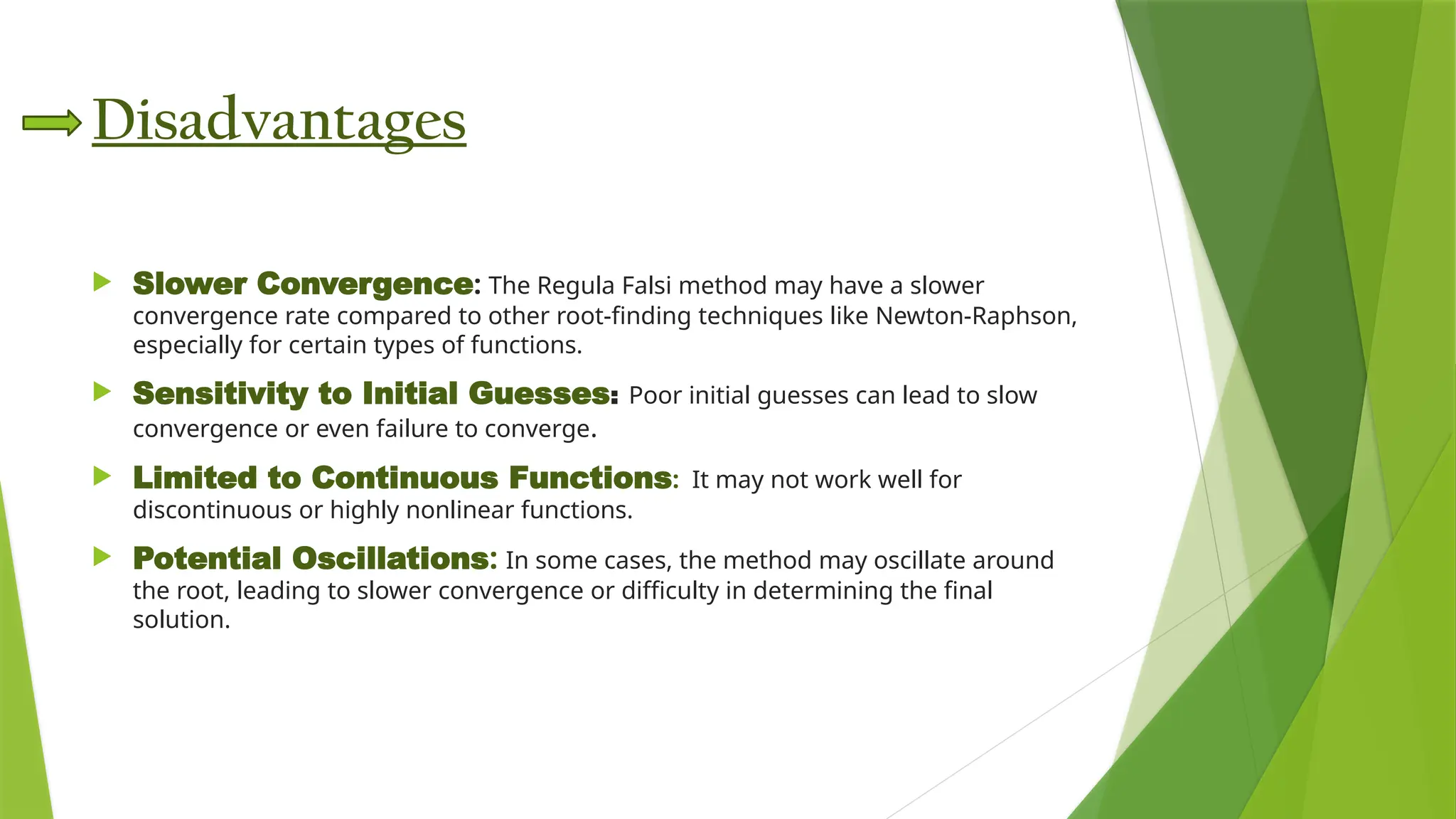
Disadvantages
Slower Convergence:The Regula Falsi method may have a slower
convergence rate compared to other root-finding techniques like Newton-Raphson,
especially for certain types of functions.
Sensitivity to Initial Guesses: Poor initial guesses can lead to slow
convergence or even failure to converge.
Limited to Continuous Functions: It may not work well for
discontinuous or highly nonlinear functions.
Potential Oscillations: In some cases, the method may oscillate around
the root, leading to slower convergence or difficulty in determining the final
solution.
6.
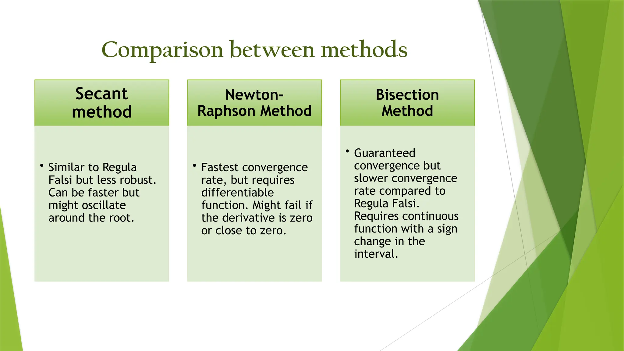
Comparison between methods
Secant
method
•Similar to Regula
Falsi but less robust.
Can be faster but
might oscillate
around the root.
Newton-
Raphson Method
• Fastest convergence
rate, but requires
differentiable
function. Might fail if
the derivative is zero
or close to zero.
Bisection
Method
• Guaranteed
convergence but
slower convergence
rate compared to
Regula Falsi.
Requires continuous
function with a sign
change in the
interval.
7.
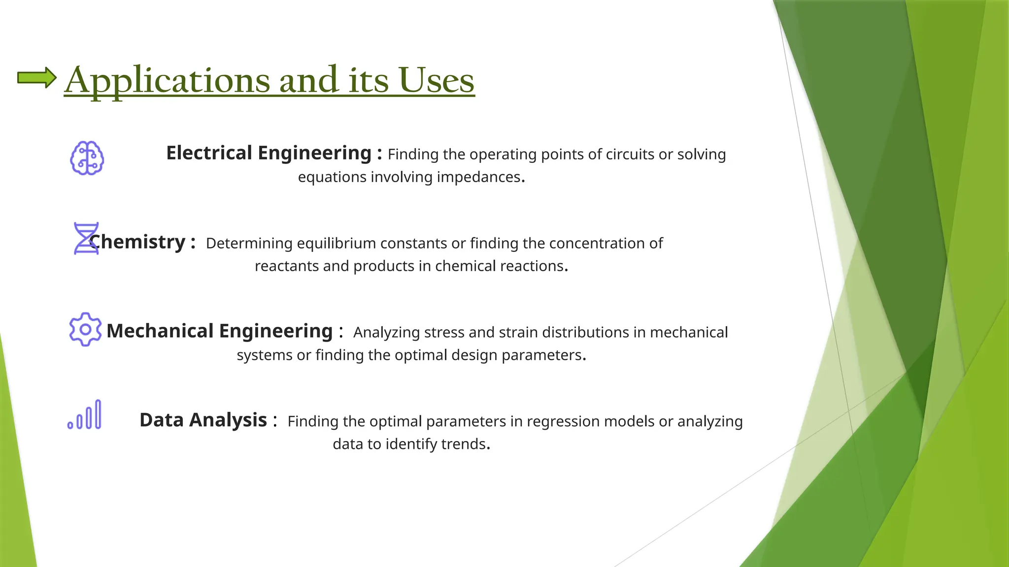
Applications and itsUses
Electrical Engineering : Finding the operating points of circuits or solving
equations involving impedances.
Chemistry : Determining equilibrium constants or finding the concentration of
reactants and products in chemical reactions.
Mechanical Engineering: Analyzing stress and strain distributions in mechanical
systems or finding the optimal design parameters.
Data Analysis: Finding the optimal parameters in regression models or analyzing
data to identify trends.
8.
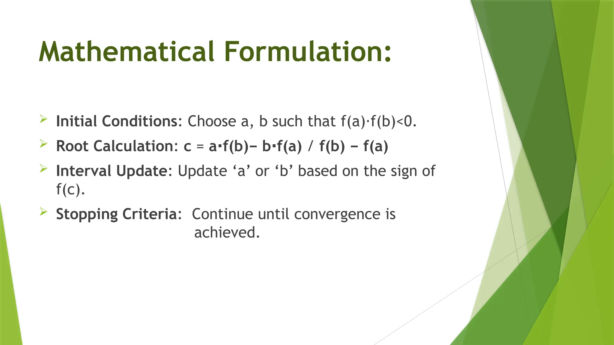
Mathematical Formulation:
InitialConditions: Choose a, b such that f(a) f(b)<0.
⋅
Root Calculation: c = a f(b)− b f(a)
⋅ ⋅ / f(b) − f(a)
Interval Update: Update ‘a’ or ‘b’ based on the sign of
f(c).
Stopping Criteria: Continue until convergence is
achieved.
9.
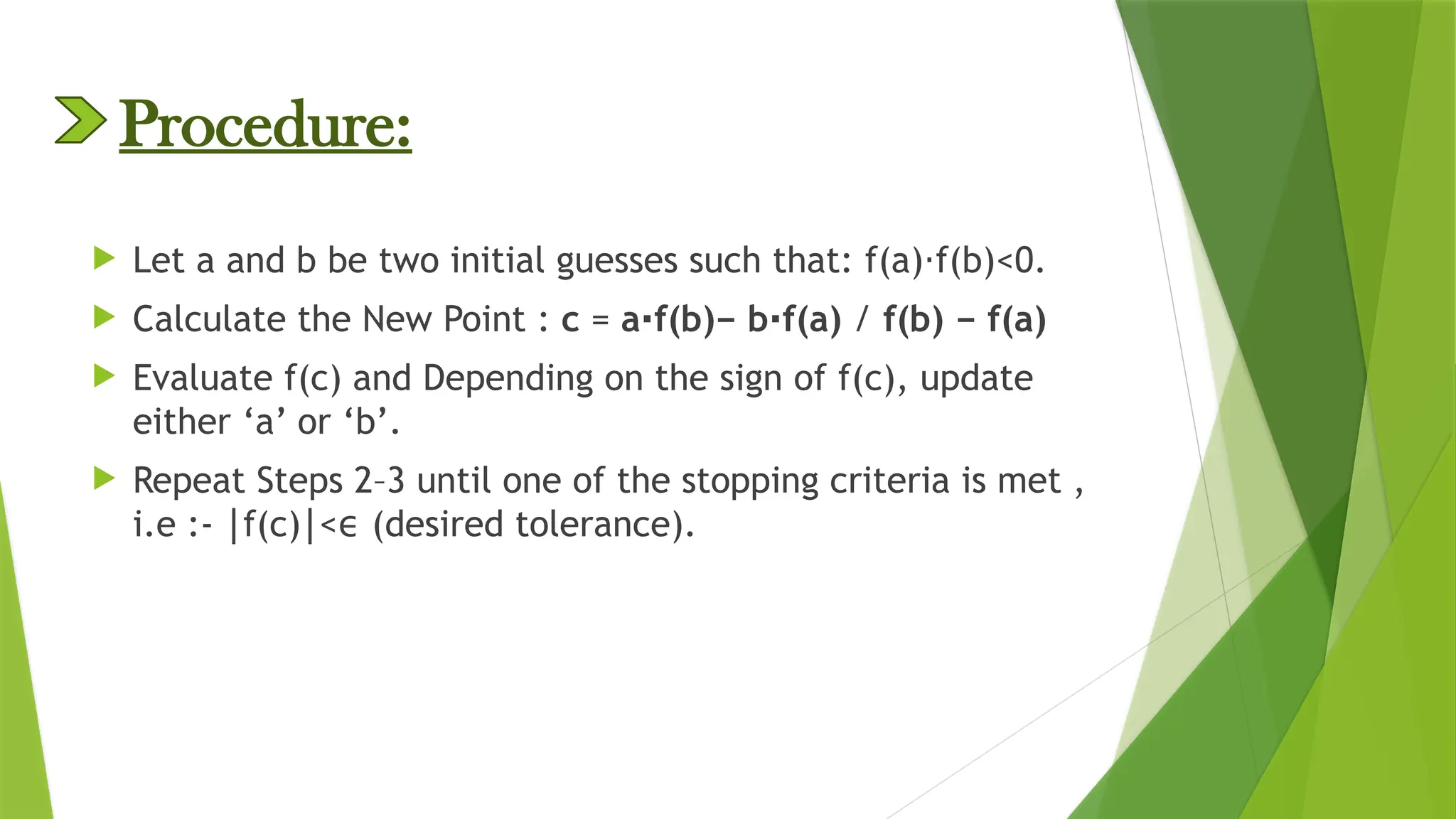
Procedure:
Let aand b be two initial guesses such that: f(a) f(b)<0.
⋅
Calculate the New Point : c = a f(b)− b f(a)
⋅ ⋅ / f(b) − f(a)
Evaluate f(c) and Depending on the sign of f(c), update
either ‘a’ or ‘b’.
Repeat Steps 2–3 until one of the stopping criteria is met ,
i.e :- f(c) < (desired tolerance).
∣ ∣ ϵ
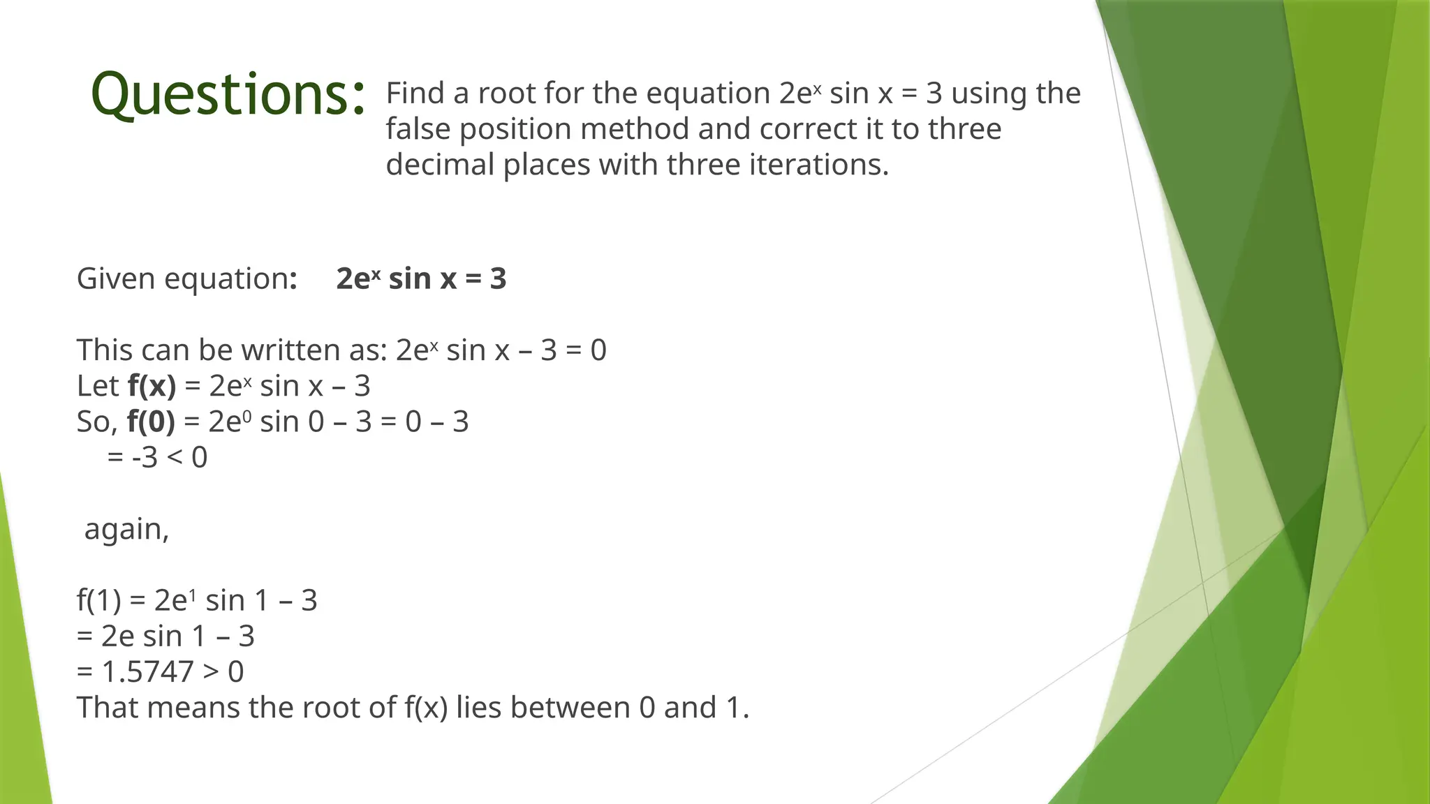
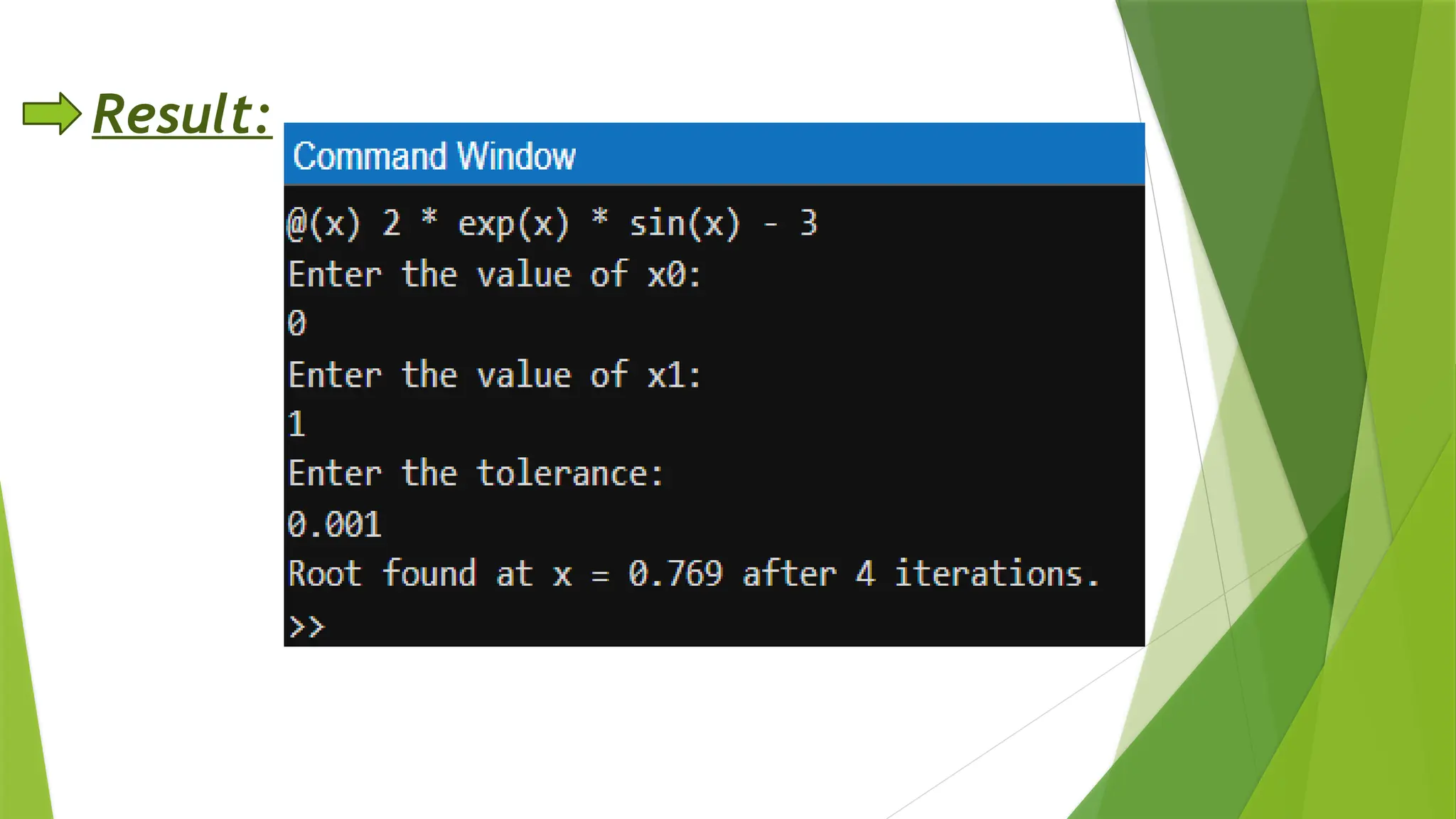
Questions: Find aroot for the equation 2ex
sin x = 3 using the
false position method and correct it to three
decimal places with three iterations.
Given equation: 2ex
sin x = 3
This can be written as: 2ex
sin x – 3 = 0
Let f(x) = 2ex
sin x – 3
So, f(0) = 2e0
sin 0 – 3 = 0 – 3
= -3 < 0
again,
f(1) = 2e1
sin 1 – 3
= 2e sin 1 – 3
= 1.5747 > 0
That means the root of f(x) lies between 0 and 1.
12.
Let a =0 and b = 1.
The first approximation = x1 = [a*f(b) – b*f(a)]/ [f(b) – f(a)]
= [0(1.5747) – 1(-3)]/ [1.5747 – (-3)]
= 3/4.5747
= 0.6557
Thus, x1 = 0.6557
Now, substitute x1 = 0.6557 in f(x).
So, f(0.6557) = 2e0.6557
sin(0.6557) – 3
= 2.3493 – 3
= -0.6507 < 0
As we know, f(1) > 0
That means a root lies between 0.6557 and 1.
13.
Let a =0.6557
The second approximation = x2 = [a*f(x1) – x1f(a)]/ [f(x1) – f(a)]
= [0.6557(1.5747) – 1(-0.6507)]/ [1.5747 – (-0.6507)]
= (1.0325 + 0.6507)/(2.2254)
= 1.6832/2.2254
= 0.7563
Therefore, x2 = 0.7563
Let us substitute 0.7563 in f(x).
So, f(0.7563) = 2e0.7563
sin(0.7563) – 3
= 2.9239 – 3
= -0.0761 < 0
We know that f(1) > 0
Thus, a root lies between 0.7563 and 1.
14.
Hence, the thirdapproximation = x3 = [a*f(x2) – x2f(a)]/ [f(x2) –
f(a)]
= [(0.7563)(1.5747) – 1(-0.0761)]/ [1.5747 – (-0.0761)]
= (1.1909 + 0.0761)/1.6508
= 1.2670/1.6508
= 0.7675
So,
x3 = 0.7675
Let us substitute 0.7675 in f(x).
So, f(0.7675) =2e0.7675
sin(0.7675) – 3
= -0.0082 < 0
15.
We know thatf(1) > 0
Thus, a root lies between a= 0.7675 and x3 = 1.
Hence, the fourth approximation =
x4 = [a*f(x3) – x3f(a)]/ [f(x3) – f(a)]
= [(0.7675)(1.5747) – 1(-0.0082)]/ [1.5747 – (-0.0082)]
=0.7687
Therefore, the best approximation of the root
up to three decimal places is 0.768
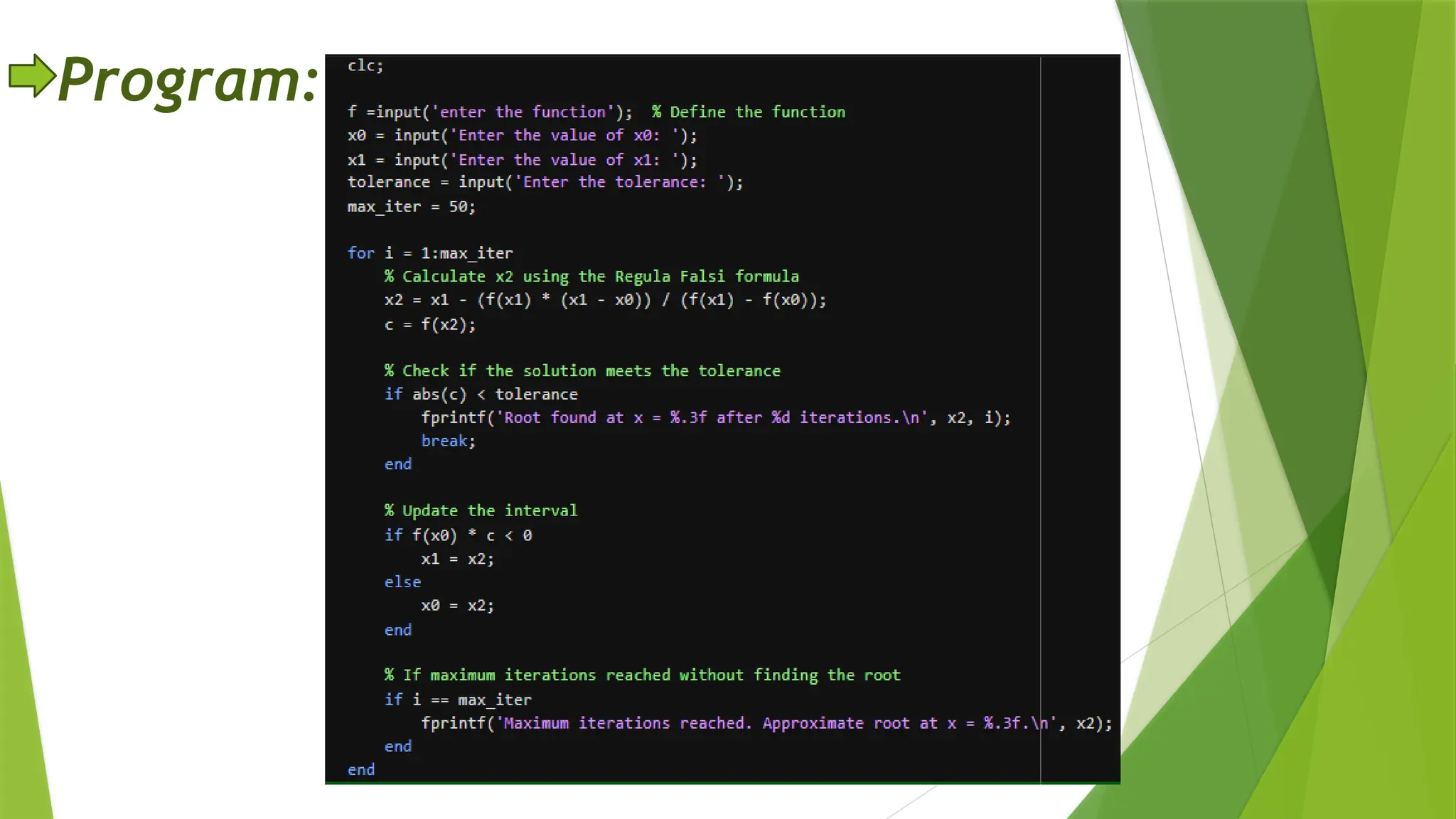
Algorithm:
Define thefunction f(x).
Choose initial guesses a and b, such that (f(a) f(b)<0) .
⋅
Check the stopping criteria, such as a predefined tolerance ,
ϵ
or maximum number of iterations.
Compute the root approximation c using the false position formula
c = (a*f(b)−b*f(a)
)/f(b)-f(a).
Update the interval based on the sign of f(c)
If f(a) f(c)<0
⋅ , then the root lies in [a,c], so set b=c.
If f(b) f(c)<0
⋅ , then the root lies in [c,b], so set a=c.
Check the convergence:
If f(c)∣is smaller than a predefined tolerance ϵ, then c is the
ϵ
root.
If not, repeat the process.
![Let a = 0 and b = 1.
The first approximation = x1 = [a*f(b) – b*f(a)]/ [f(b) – f(a)]
= [0(1.5747) – 1(-3)]/ [1.5747 – (-3)]
= 3/4.5747
= 0.6557
Thus, x1 = 0.6557
Now, substitute x1 = 0.6557 in f(x).
So, f(0.6557) = 2e0.6557
sin(0.6557) – 3
= 2.3493 – 3
= -0.6507 < 0
As we know, f(1) > 0
That means a root lies between 0.6557 and 1.](https://image.slidesharecdn.com/regulafalsimethod-250807181809-8f3f38c4/75/REGULA-FALSI-METHOD-numerical-methods-12-2048.jpg)
![Let a = 0.6557
The second approximation = x2 = [a*f(x1) – x1f(a)]/ [f(x1) – f(a)]
= [0.6557(1.5747) – 1(-0.6507)]/ [1.5747 – (-0.6507)]
= (1.0325 + 0.6507)/(2.2254)
= 1.6832/2.2254
= 0.7563
Therefore, x2 = 0.7563
Let us substitute 0.7563 in f(x).
So, f(0.7563) = 2e0.7563
sin(0.7563) – 3
= 2.9239 – 3
= -0.0761 < 0
We know that f(1) > 0
Thus, a root lies between 0.7563 and 1.](https://image.slidesharecdn.com/regulafalsimethod-250807181809-8f3f38c4/75/REGULA-FALSI-METHOD-numerical-methods-13-2048.jpg)
![Hence, the third approximation = x3 = [a*f(x2) – x2f(a)]/ [f(x2) –
f(a)]
= [(0.7563)(1.5747) – 1(-0.0761)]/ [1.5747 – (-0.0761)]
= (1.1909 + 0.0761)/1.6508
= 1.2670/1.6508
= 0.7675
So,
x3 = 0.7675
Let us substitute 0.7675 in f(x).
So, f(0.7675) =2e0.7675
sin(0.7675) – 3
= -0.0082 < 0](https://image.slidesharecdn.com/regulafalsimethod-250807181809-8f3f38c4/75/REGULA-FALSI-METHOD-numerical-methods-14-2048.jpg)
![We know that f(1) > 0
Thus, a root lies between a= 0.7675 and x3 = 1.
Hence, the fourth approximation =
x4 = [a*f(x3) – x3f(a)]/ [f(x3) – f(a)]
= [(0.7675)(1.5747) – 1(-0.0082)]/ [1.5747 – (-0.0082)]
=0.7687
Therefore, the best approximation of the root
up to three decimal places is 0.768](https://image.slidesharecdn.com/regulafalsimethod-250807181809-8f3f38c4/75/REGULA-FALSI-METHOD-numerical-methods-15-2048.jpg)
![Algorithm:
Define the function f(x).
Choose initial guesses a and b, such that (f(a) f(b)<0) .
⋅
Check the stopping criteria, such as a predefined tolerance ,
ϵ
or maximum number of iterations.
Compute the root approximation c using the false position formula
c = (a*f(b)−b*f(a)
)/f(b)-f(a).
Update the interval based on the sign of f(c)
If f(a) f(c)<0
⋅ , then the root lies in [a,c], so set b=c.
If f(b) f(c)<0
⋅ , then the root lies in [c,b], so set a=c.
Check the convergence:
If f(c)∣is smaller than a predefined tolerance ϵ, then c is the
ϵ
root.
If not, repeat the process.](https://image.slidesharecdn.com/regulafalsimethod-250807181809-8f3f38c4/75/REGULA-FALSI-METHOD-numerical-methods-17-2048.jpg)


![[DSC Europe 25] Branko Dzakula - From Defense to Attack: How AI Redefines Cyb...](https://cdn.slidesharecdn.com/ss_thumbnails/80bdzdxpr3ky2g0qvyk9-8-251211083048-ce5fc1ee-thumbnail.jpg?width=640&height=640&fit=bounds)


![[DSC Europe 25] Jon Dajci - Bridging TradFi and DeFi: Building the Future of ...](https://cdn.slidesharecdn.com/ss_thumbnails/fqmhfvlbqhkihjvqvhmu-7-251211083849-6af7e325-thumbnail.jpg?width=640&height=640&fit=bounds)

