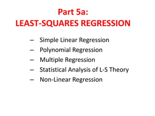
Part 5a:
LEAST-SQUARES REGRESSION
–
–
–
–
–

Simple Linear Regression
Polynomial Regression
Multiple Regression
Statistical Analysis of L-S Theory
Non-Linear Regression
Introduction:
Consider the falling object in air problem:
t0

m

v0

t1

m

“Best fit”

v1

v

t

tn

m

vn

 (t) values considered to be error-free.
 Every measurement of (v) contain some error.
 Assume error in (v) are normally distributed
(random error).
 Find “best fit” curve to represent v(t)
Simple Linear Regression
 Consider a set of n scattered data
 Find a line that “best fits” the scattered data
y

a0

a0= intercept
a1= slope

a1 x

 There are a number of ways to define the “best fit” line. However
we want to find one that is unique, i.e., for a particular set of data.
 A uniquely defined best-fit line can be found by minimizing the
sum of the square of the residuals from each data point:
n

Sr

n

( ymeas
i 1

y fit ) 2

( yi

a0 a1 xi ) 2

i 1

Find a0 and a1 that minimizes Sr (least-square)

sum of the square
of the residuals
(or spread)
To minimize Sr (a0 , a1), differentiate and set to zero:
n

Sr
a0

2

( yi

a0

a1 xi )

0

[( yi

a0

a1 xi ) xi ] 0

i 1
n

Sr
a1

2
i 1

or
0
na0
xi a0

yi

a0
xi a1
xi2 a1

a1xi
yi

0

yi xi

a0 xi

a1 xi2

Normal equations for
simple linear L-S regression

xi yi

Need to solve these simultaneous equations for the unknowns a0
and a1
Solution for a1 and a0 gives
n

a1

xi yi
n

xi

2
i

x

xi

yi
2

and

yi

a0

n

xi

a1

n

y a1 x

EX: Find linear fit for the set of measurements:
x
1

0.5

2

2.5

3

2.0

4

4.0

5

3.5

6

6.0

7

y

y

5.5

0.0714 0.839x

n 7

xi

28

x 4
xi yi 119.5

a1
a0

yi
y

3.4286

xi2 140

7(119 .5) 2(24 )
7(140 ) (28 ) 2
3.4286

24

0.839 (4)

0.839
0.0714
Quantification of Error:
Sum of the square of the
residuals for the mean
2

n

St

sum of the square of the
residuals for the linear
regression

( yi

y)

Sr

( yi

a0 a1 xi )

i 1

i 1

standard
deviation

sy

2

n

St
n 1

standard error of
the L-S estimate

sy/ x

Sr
n 2

All these
approaches are
based on the
assumptions:
x > error-free
y > normal error
“Coefficient of determination” is defined as
r

St

2

Sr

r

St

Sr =0 (r=1)
Sr =St (r=0)

“correlation coefficient”

Perfect fit
No improvement by fitting the line

Alternative formulation for the correlation coefficient
n

r
n

2
i

x

xi yi
xi

xi
2

n

yi
2
i

y

yi

Note: r 1 does not always necessarily mean
that the fit is “good”. You should always plot
the data along with the regression curve to
see the goodness of the fit.

2

Four set of data with same r=0.816
Linearization of non-linear relationships:
 Many engineering applications involve non-linear
relationships, e.g., exponential, power law, or saturated growth
rate.
exponential
power-law
saturated growth-rate
y

a1e b1x

y

a2 x b2

y

a3

x
b3

x

 These relationships can be linearized by some mathematical
operations:
ln y

ln a1 b1 x

log y

b2 log x log a2

1
y

b3 1
a3 x

 Linear L-S fit can be applied to find the coefficients.

1
a3
EX: Fit a power law relationship to the following dataset:
x

y

1

0.5

2

1.7

3

3.4

4

5.7

5

8.4

Power law model

y

log y

a2 x b2

b2 log x log a2

(find a2 and b2)
Calculate logarithm of both data:
log x

log y

0

-0.301

0.301

0.226

0.477

0.534

0.602

0.753

0.699

0.922

Applying simple linear regression gives;
slope=1.75 and intercept=-0.300

b2

1.75 log a2
y

0.5 x1.75

0.300

a2

0.5
Polynomial Regression
 In some cases, we may want to fit our data to a curve rather than a
line. We can then apply polynomial regression (In fact, linear
regression is nothing but an n=1 polynomial regression).

Data to fit to a second order polynomial:
y

a0

a1 x a2 x 2

Sum of the square of the residuals (spread)
2

n

Sr

( yi ,obs

yi , fit )

i 1

2

n

( yi a0 a1 xi

a2 xi2 )

i 1

To minimize Sr(a0, a1, a2), take derivatives and equate to zero:
Sr
a0

n

2

( yi
i 1

a0

a1 xi

a2 xi2 )

0
Sr
a1
Sr
a2

n

xi ( yi

a0

a1 xi

a2 xi2 )

0

xi2 ( yi

2

a0

a1 xi

a2 xi2 )

0

i 1
n

2
i 1

Three linear equations with three unknowns a0, a1, a2 :
(n)a0

xi a1

xi2 a2

yi

xi a0

xi2 a1

xi3 a2

xi yi

“normal equations”

xi2 a0

xi3 a1

xi4 a2

xi2 yi

all summations are i=1..n

 This set of equations can be solved by any linear solution
techniques (e.g., Gauss elimination, LU Dec., Cholesky Dec., etc.)
 The approach can be generalized to order (m) polynomial following
the same way. Now, the fit function becomes
y

a1 x a2 x 2 .. am x m

a0

 This will require the solution of an order (m+1) system of linear
equations. The standard error becomes
Because (m+1) degrees of
freedom was lost from data
of (n) due to extraction of
(m+1) coefficients .

Sr
n (m 1)

sy / x

EX 17.5: Fit an 2nd order polynomial to the following data x
i

yi 152.6

m 2
2
i

x

55

xi yi
xi2 yi

3
i

x

225

2488.8
4
i

x

979

2.1
7.7

2

13.6

3

585.6

0
1

xi 15

n 6

yi

27.2

4

40.9

5

61.1
System of linear equations:

6

15

55

a0

152.6

15

55

225 a1

585.6

55 225 979 a2

2488.8

We get

a0

2.47857

a1

2.35929

a2

1.86071

Then, the fit function:

y

2.47857

2.35929 x 1.86071 x 2

Standard error:

Sr
n (m 1)

sy / x
where

3.74657
1.12
6 (3)
2

6

Sr

( yi
i 1

2.47857 2.35929xi 1.86071xi2 )

3.74657
Multiple Linear Regression
 In some cases, data may
have two or more
independent variables. In
this example, for a
function of two
x 2 variables, the linear
regression gives a planar fit
function.

y ( x1 , x2 )

x1

Function to fit
y

a0

a1 x1 a2 x2

Sum of the square of the residuals (spread)
2

n

Sr

( yi ,obs
i 1

2

n

yi , fit )

( yi a0 a1 x1i a2 x2i )
i 1
Minimizing the spread function gives:
n

Sr
a0

2

( yi

a0

a1 x1i

a 2 x2 i )

0

i 1
n

Sr
a1

2

x1i ( yi

a0

a1 x1i

a 2 x2 i )

0

x2 i ( yi

a0

a1 x1i

a 2 x2 i )

0

i 1
n

Sr
a2

2
i 1

The system of equations to be solved:
n

x1i
2
1i

x1i

x

x2 i

x1i x2i

x2 i

a0

yi

x1i x2i

a1

x1i y1i

2
x2 i

a2

x 2 i yi

Normal equations
for multiple linear
regression
EX 17.7: Fit a planar surface to the following data
x1

x2

y

0

0

5

2

1

10

2.5

2

9

1

3

0

4

6

3

7

2

27

We first do the following calculations:
y

x1

x2

x1x1

x2x2

x1x2

x1y

x2y

5

0

5

0

0

0

0

0

10

1

10

4

1

2

20

10

9

2

9

6.25

4

5

22.5

18

0

3

0

1

9

3

0

0

3

6

3

16

36

24

12

18

27

2

27

49

4

14

189

54

54

16.5

14

76.25

54

48

243.5

100
The system of equations to calculate the fit coefficients:

6

16.5

14 a0

16.5 76.25 48 a1
14

48

54 a2

54
243.5
100

returns

a0

a1

5

The fit function

y

4

a2

3

5 4 x1 3x2

 For the general case of a function of m-variables, the same
strategy can applied. The fit function in this case:
y a0 a1 x1 a2 x2 .. am xm

Standard error:
sy / x

Sr
n (m 1)
 A useful application of multiple regression is for fitting a power
law equation of multiple variables of the form:
y

a
a
a0 x1a1 x2 2 .. xmm

Linearization of this equation gives
log y

log a0

a1 log x1 ... am log xm

 The coefficients in the last equation can be calculated using
multiple linear regression, and can be substituted to the original
power law equation.
Generalization of L-S Regression:
 In the most general form, L-S regression can be stated as
y

a0 z0

a1 z1 ... am zm

In general, this form is called
“linear regression” as the
fitting coefficients are
linearly dependant on the fit
function.

functions

z0

x 0 , z1

z0

1 , z1

x1 , ..., z m

x1 , ..., zm

xm

xm

Polynomial regression
Multiple regression

 Other functions can be defined for fitting as well, e.g.,
y

a0

a1 cos t a2 sin t
For a particular data point
y

a0 z0

a1 z1 ... am zm

e

data

For n data (in matrix form):
y

z10
Z

Z a

e

y1
y2
...
yn

coefficients

a0
a1
...
am

residuals

z11 ... z1m

...
...
zn 0

y

a

e

Calculated based on the
measured independant
variables

zn1

znm

m: order of the fit function
n: number of data points
Z is generally not a square matrix.

n m 1

e1
e2
...
en
Sum of the square of the residuals:
n

2

m

Sr

( yi
i 1

a j z ji )
j 0

To determine the fit coefficients, minimize

S r (a0 , a1 ,.., am )

This is equivalent to the following:
Z

T

Z a

Z

T

y

Normal equations
for the general L-S
regression

 This is the general representation of the normal equations for L-S
regression including simple linear, polynomial, and multiple linear
regression methods.
Solution approaches:
Z

T

Z a

Z

T

y

A symmetric and square
matrix of size [m+1 , m+1]

 Elimination methods are best suited for the solution of the above
linear system:
LU Decomposition / Gauss Elimination
Cholesky Decomposition
 Especially, Cholesky decomposition is fast and requires less
storage. Furthermore,
 Cholesky decomposition is very appropriate when the order of
the polynomial fit model (m) is not known beforehand.
Successive higher order models can be efficiently developed.
 Similarly, increasing the number of variables in multiple
regression is very efficient using Cholesky decomposition.
Statistical Analysis of L-S Theory
Some definitions:

 If a histogram of the data shows a
bell shape curve, normally
distributed data.
 This has a well-defined statistics

n

yi
y

sy

2
sy

mean

i 1

n
yi
n 1

St
n 1

y

2

Standard
deviation
variance

 For a perfectly normal distribution:
mean±std fall about 68% of the total data.
mean±2std fall about 95% of the total data.

: true mean
: true std
Confidence intervals:
 Confidence interval estimates intervals within which the
parameter is expected to fall, with a certain degree of confidence.
 Find L and U values such that
PL

U

1

true mean

significance level
For 95% confidence interval
=0.05
L

U

y

y

sy
n

sy
n

t

t

/ 2,n 1

/ 2,n 2

t-distribution (tabulated in
books); in EXCEL tinv ( ,n)

e.g., for =0.05 and n=20
t /2, n-1=2.086

 T-distribution is used to compramize between a
perfect and an imperfect estimate. For example, if
data is few (small n), t-value becomes larger, hence
giving a more conservative interval of confidence.
EX: Some measurements of coefficient of thermal expansion of steel (x10-6 1/°F):
6.495
6.665
6.755
6.565

6.595
6.505
6.625
6.515

6.615
6.435
6.715
6.555

6.635
6.625
6.575
6.395

6.485
6.715
6.655
6.775

6.555
6.655
6.605
6.685

n=8
n=16

n=24

Find the mean and corresponding 95% confidence intervals for the
a) first 8 measurements b) first 16 measurements c) all 24 measurements.
For n=8

L

y

U

y

y
sy
n

sy
n

6.59
t

t

sy

0.089921

t

/ 2,n 1

t0.05 / 2,8

/ 2,n 1

6.59

0.089921
2.364623
8

/ 2,n 2

0.089921
2.364623
8

6.6652

2.364623

6.5148

6.59

1

6.5148

6.6652

For eight measurements,
there is a 95% probability
that true mean falls
between these values.
The cases of n=16 and n=24 can be performed in a similar fashion. Hence we
obtain:
n

mean(y)

8

6.5900

16
24

sy

t

L

U

0.089921 2.364623

6.5148

6.6652

6.5794

0.095845 2.131451

6.5283

6.6304

6.6000

0.097133 2.068655

6.5590

6.6410

/2,n-1

Results shows that confidence interval narrows down as the number of
measurements increases (even though sy increases by increasing n!).
For n=24 we have 95% confidence that true mean is between 6.5590 and 6.6410.
Confidence Interval for L-S regression:
 Using matrix inverse for the solution of (a) is inefficient:
a

Z

T

Z

1

Z

T

y

 However, inverse matrix carries useful statistical information
about the goodness of the fit.
Z

T

Z

1

Inverse matrix

Diagonal terms
coefficients

variances (var) of the fit

Off -diagonal terms
the fit coefficients

covariances (cov) of

2
var(ai 1 ) uii s y / x

cov(ai 1, a j ) ui

2
sy / x
1, j

uij: Elements of the inverse matrix

 These statistics allow calculation of confidence intervals for the
fit coefficients.
 Calculating confidence intervals for simple linear regression:
y

a0

a1 x

For the intercept (a0)
L

a0 t

/ 2,n 2

s ( a0 )

U

a0 t

/ 2,n 2

s ( a0 )

For the slope (a1)
L

a1 t

U

a1 t

/ 2,n 2

s (a1 )

/ 2,n 2

s (a1 )

Standard error for the coefficient
(extracted from the inverse matrix)

s(ai )

var(ai )
EX 17.8: Compare results of measured versus model data shown below.
a) Plot the measured versus model values.
b) Apply simple linear regression formula to see the adequacy of the measured
versus model data.
c) Recompute regression using matrix approach, estimate standard error of the
estimation and for the fit parameters, and develop confidence intervals.
a)
60
Model
value
8.953
16.405
22.607
27.769
32.065
35.641
38.617
41.095
43.156
44.872
46.301
47.49
48.479
49.303
49.988

50
40

model

Measured
Value
10
16.3
23
27.5
31
35.6
39
41.5
42.9
45
46
45.5
46
49
50

30
20
10
0

0

20

40

60

measured

b) Applying simple linear regression formula gives

y

0.859 1.032x

x: measured
y: model
c) For the statistical analysis, first form the following [Z] matrix and (y) vector

1
Z

Then,

10

8.953

1 16.3
.. ..
..
1

16.405
..

y

..
50
Z

..
49.988
T

T

Z a

Z

548.3

a0

552.741

548.3 22191.21 a1

22421.43

15

y

Solution using the matrix inversion

a
a0
a1

0.688414

Z

T

Z

1

Z

0.01701

T

y

552.741

0.85872

0.01701 0.000465 22421.43

1.031592
Standard error for the fit function:

Sr
n 2

sy / x

0.863403

Standard error for the coefficients:

s(a0 )

2
u11s y / x

0.688414(0.863403) 2

0.716372

s(a1 )

2
u22 s y / x

0.000465(0.863403) 2

0.018625

For a 95% confidence interval ( =0.05, n=13, Excel returns inv(0.05,13)=2.160368)

a0

a0 t

/ 2, n 2

s(a0 )

0.85872 2.160368(0.716372)
0.85872 1.547627

a1

a1 t

/ 2, n 2

s(a1 ) 1.031592 2.160368(0.018625)
1.031592 0.040237

Desired values of slope=1 and intercept=0 falls in the intervals (hence we can
conclude that a good fit exist between measured and model values).
Non-linear Regression
 In some cases we must fit a non-linear model to the data, e.g.,
y

a0 (1 e

a1 x

)

parameters a0 and a1
are not linearly
dependant on y

 Generalized L-S formulation cannot be used for such models.
 Same approach of using sum of square of the residuals are
applied, but the solution is sought iteratively.
Gauss-Newton method:
 A Taylor series expansion is used to (approximately) linearize the
model. Then standard L-S theory can be applied to estimate the
improved estimates of the fit parameters.
In most general form
y

f ( x; a0 , a1 ,..am )
Taylor series around the fit parameters
f ( xi ) j

f ( xi ) j

f ( xi )

1

a0

f ( xi ) j

a0

a1

i: i-th data point
j: iteration number

a1

Then
ymeas

f ( xi ) j

y fit

a0

a0

f ( xi ) j
a1

a1

In matrix form:
d

Zj

iteration number

d

a

y1

f ( x1 )

y2

f ( x2 )
...

yn

f ( xn )

Zj

f1
a0
f2
a0
...
fn
a0

f1
a0
f2
a0
...
fn
a0

a

a0
a1
Applying the generalized L-S formula
Zj

T

Zj

a

Zj

T

d

 We solve the above system for ( A) for improved values of
parameters:
a0 , j

1

a0 , j

a0

a1, j

1

a1, j

a1

 The procedure is iterated until an acceptable error:
a0 , j
a 0

1

a0 , j

a0 , j

a1, j
a 1

1

1

a1, j

a1, j
1

Es272 ch5a

  • 1.
    Part 5a: LEAST-SQUARES REGRESSION – – – – – SimpleLinear Regression Polynomial Regression Multiple Regression Statistical Analysis of L-S Theory Non-Linear Regression
  • 2.
    Introduction: Consider the fallingobject in air problem: t0 m v0 t1 m “Best fit” v1 v t tn m vn  (t) values considered to be error-free.  Every measurement of (v) contain some error.  Assume error in (v) are normally distributed (random error).  Find “best fit” curve to represent v(t)
  • 3.
    Simple Linear Regression Consider a set of n scattered data  Find a line that “best fits” the scattered data y a0 a0= intercept a1= slope a1 x  There are a number of ways to define the “best fit” line. However we want to find one that is unique, i.e., for a particular set of data.  A uniquely defined best-fit line can be found by minimizing the sum of the square of the residuals from each data point: n Sr n ( ymeas i 1 y fit ) 2 ( yi a0 a1 xi ) 2 i 1 Find a0 and a1 that minimizes Sr (least-square) sum of the square of the residuals (or spread)
  • 4.
    To minimize Sr(a0 , a1), differentiate and set to zero: n Sr a0 2 ( yi a0 a1 xi ) 0 [( yi a0 a1 xi ) xi ] 0 i 1 n Sr a1 2 i 1 or 0 na0 xi a0 yi a0 xi a1 xi2 a1 a1xi yi 0 yi xi a0 xi a1 xi2 Normal equations for simple linear L-S regression xi yi Need to solve these simultaneous equations for the unknowns a0 and a1
  • 5.
    Solution for a1and a0 gives n a1 xi yi n xi 2 i x xi yi 2 and yi a0 n xi a1 n y a1 x EX: Find linear fit for the set of measurements: x 1 0.5 2 2.5 3 2.0 4 4.0 5 3.5 6 6.0 7 y y 5.5 0.0714 0.839x n 7 xi 28 x 4 xi yi 119.5 a1 a0 yi y 3.4286 xi2 140 7(119 .5) 2(24 ) 7(140 ) (28 ) 2 3.4286 24 0.839 (4) 0.839 0.0714
  • 6.
    Quantification of Error: Sumof the square of the residuals for the mean 2 n St sum of the square of the residuals for the linear regression ( yi y) Sr ( yi a0 a1 xi ) i 1 i 1 standard deviation sy 2 n St n 1 standard error of the L-S estimate sy/ x Sr n 2 All these approaches are based on the assumptions: x > error-free y > normal error
  • 7.
    “Coefficient of determination”is defined as r St 2 Sr r St Sr =0 (r=1) Sr =St (r=0) “correlation coefficient” Perfect fit No improvement by fitting the line Alternative formulation for the correlation coefficient n r n 2 i x xi yi xi xi 2 n yi 2 i y yi Note: r 1 does not always necessarily mean that the fit is “good”. You should always plot the data along with the regression curve to see the goodness of the fit. 2 Four set of data with same r=0.816
  • 8.
    Linearization of non-linearrelationships:  Many engineering applications involve non-linear relationships, e.g., exponential, power law, or saturated growth rate. exponential power-law saturated growth-rate y a1e b1x y a2 x b2 y a3 x b3 x  These relationships can be linearized by some mathematical operations: ln y ln a1 b1 x log y b2 log x log a2 1 y b3 1 a3 x  Linear L-S fit can be applied to find the coefficients. 1 a3
  • 9.
    EX: Fit apower law relationship to the following dataset: x y 1 0.5 2 1.7 3 3.4 4 5.7 5 8.4 Power law model y log y a2 x b2 b2 log x log a2 (find a2 and b2) Calculate logarithm of both data: log x log y 0 -0.301 0.301 0.226 0.477 0.534 0.602 0.753 0.699 0.922 Applying simple linear regression gives; slope=1.75 and intercept=-0.300 b2 1.75 log a2 y 0.5 x1.75 0.300 a2 0.5
  • 10.
    Polynomial Regression  Insome cases, we may want to fit our data to a curve rather than a line. We can then apply polynomial regression (In fact, linear regression is nothing but an n=1 polynomial regression). Data to fit to a second order polynomial: y a0 a1 x a2 x 2 Sum of the square of the residuals (spread) 2 n Sr ( yi ,obs yi , fit ) i 1 2 n ( yi a0 a1 xi a2 xi2 ) i 1 To minimize Sr(a0, a1, a2), take derivatives and equate to zero: Sr a0 n 2 ( yi i 1 a0 a1 xi a2 xi2 ) 0
  • 11.
    Sr a1 Sr a2 n xi ( yi a0 a1xi a2 xi2 ) 0 xi2 ( yi 2 a0 a1 xi a2 xi2 ) 0 i 1 n 2 i 1 Three linear equations with three unknowns a0, a1, a2 : (n)a0 xi a1 xi2 a2 yi xi a0 xi2 a1 xi3 a2 xi yi “normal equations” xi2 a0 xi3 a1 xi4 a2 xi2 yi all summations are i=1..n  This set of equations can be solved by any linear solution techniques (e.g., Gauss elimination, LU Dec., Cholesky Dec., etc.)
  • 12.
     The approachcan be generalized to order (m) polynomial following the same way. Now, the fit function becomes y a1 x a2 x 2 .. am x m a0  This will require the solution of an order (m+1) system of linear equations. The standard error becomes Because (m+1) degrees of freedom was lost from data of (n) due to extraction of (m+1) coefficients . Sr n (m 1) sy / x EX 17.5: Fit an 2nd order polynomial to the following data x i yi 152.6 m 2 2 i x 55 xi yi xi2 yi 3 i x 225 2488.8 4 i x 979 2.1 7.7 2 13.6 3 585.6 0 1 xi 15 n 6 yi 27.2 4 40.9 5 61.1
  • 13.
    System of linearequations: 6 15 55 a0 152.6 15 55 225 a1 585.6 55 225 979 a2 2488.8 We get a0 2.47857 a1 2.35929 a2 1.86071 Then, the fit function: y 2.47857 2.35929 x 1.86071 x 2 Standard error: Sr n (m 1) sy / x where 3.74657 1.12 6 (3) 2 6 Sr ( yi i 1 2.47857 2.35929xi 1.86071xi2 ) 3.74657
  • 14.
    Multiple Linear Regression In some cases, data may have two or more independent variables. In this example, for a function of two x 2 variables, the linear regression gives a planar fit function. y ( x1 , x2 ) x1 Function to fit y a0 a1 x1 a2 x2 Sum of the square of the residuals (spread) 2 n Sr ( yi ,obs i 1 2 n yi , fit ) ( yi a0 a1 x1i a2 x2i ) i 1
  • 15.
    Minimizing the spreadfunction gives: n Sr a0 2 ( yi a0 a1 x1i a 2 x2 i ) 0 i 1 n Sr a1 2 x1i ( yi a0 a1 x1i a 2 x2 i ) 0 x2 i ( yi a0 a1 x1i a 2 x2 i ) 0 i 1 n Sr a2 2 i 1 The system of equations to be solved: n x1i 2 1i x1i x x2 i x1i x2i x2 i a0 yi x1i x2i a1 x1i y1i 2 x2 i a2 x 2 i yi Normal equations for multiple linear regression
  • 16.
    EX 17.7: Fita planar surface to the following data x1 x2 y 0 0 5 2 1 10 2.5 2 9 1 3 0 4 6 3 7 2 27 We first do the following calculations: y x1 x2 x1x1 x2x2 x1x2 x1y x2y 5 0 5 0 0 0 0 0 10 1 10 4 1 2 20 10 9 2 9 6.25 4 5 22.5 18 0 3 0 1 9 3 0 0 3 6 3 16 36 24 12 18 27 2 27 49 4 14 189 54 54 16.5 14 76.25 54 48 243.5 100
  • 17.
    The system ofequations to calculate the fit coefficients: 6 16.5 14 a0 16.5 76.25 48 a1 14 48 54 a2 54 243.5 100 returns a0 a1 5 The fit function y 4 a2 3 5 4 x1 3x2  For the general case of a function of m-variables, the same strategy can applied. The fit function in this case: y a0 a1 x1 a2 x2 .. am xm Standard error: sy / x Sr n (m 1)
  • 18.
     A usefulapplication of multiple regression is for fitting a power law equation of multiple variables of the form: y a a a0 x1a1 x2 2 .. xmm Linearization of this equation gives log y log a0 a1 log x1 ... am log xm  The coefficients in the last equation can be calculated using multiple linear regression, and can be substituted to the original power law equation.
  • 19.
    Generalization of L-SRegression:  In the most general form, L-S regression can be stated as y a0 z0 a1 z1 ... am zm In general, this form is called “linear regression” as the fitting coefficients are linearly dependant on the fit function. functions z0 x 0 , z1 z0 1 , z1 x1 , ..., z m x1 , ..., zm xm xm Polynomial regression Multiple regression  Other functions can be defined for fitting as well, e.g., y a0 a1 cos t a2 sin t
  • 20.
    For a particulardata point y a0 z0 a1 z1 ... am zm e data For n data (in matrix form): y z10 Z Z a e y1 y2 ... yn coefficients a0 a1 ... am residuals z11 ... z1m ... ... zn 0 y a e Calculated based on the measured independant variables zn1 znm m: order of the fit function n: number of data points Z is generally not a square matrix. n m 1 e1 e2 ... en
  • 21.
    Sum of thesquare of the residuals: n 2 m Sr ( yi i 1 a j z ji ) j 0 To determine the fit coefficients, minimize S r (a0 , a1 ,.., am ) This is equivalent to the following: Z T Z a Z T y Normal equations for the general L-S regression  This is the general representation of the normal equations for L-S regression including simple linear, polynomial, and multiple linear regression methods.
  • 22.
    Solution approaches: Z T Z a Z T y Asymmetric and square matrix of size [m+1 , m+1]  Elimination methods are best suited for the solution of the above linear system: LU Decomposition / Gauss Elimination Cholesky Decomposition  Especially, Cholesky decomposition is fast and requires less storage. Furthermore,  Cholesky decomposition is very appropriate when the order of the polynomial fit model (m) is not known beforehand. Successive higher order models can be efficiently developed.  Similarly, increasing the number of variables in multiple regression is very efficient using Cholesky decomposition.
  • 23.
    Statistical Analysis ofL-S Theory Some definitions:  If a histogram of the data shows a bell shape curve, normally distributed data.  This has a well-defined statistics n yi y sy 2 sy mean i 1 n yi n 1 St n 1 y 2 Standard deviation variance  For a perfectly normal distribution: mean±std fall about 68% of the total data. mean±2std fall about 95% of the total data. : true mean : true std
  • 24.
    Confidence intervals:  Confidenceinterval estimates intervals within which the parameter is expected to fall, with a certain degree of confidence.  Find L and U values such that PL U 1 true mean significance level For 95% confidence interval =0.05 L U y y sy n sy n t t / 2,n 1 / 2,n 2 t-distribution (tabulated in books); in EXCEL tinv ( ,n) e.g., for =0.05 and n=20 t /2, n-1=2.086  T-distribution is used to compramize between a perfect and an imperfect estimate. For example, if data is few (small n), t-value becomes larger, hence giving a more conservative interval of confidence.
  • 25.
    EX: Some measurementsof coefficient of thermal expansion of steel (x10-6 1/°F): 6.495 6.665 6.755 6.565 6.595 6.505 6.625 6.515 6.615 6.435 6.715 6.555 6.635 6.625 6.575 6.395 6.485 6.715 6.655 6.775 6.555 6.655 6.605 6.685 n=8 n=16 n=24 Find the mean and corresponding 95% confidence intervals for the a) first 8 measurements b) first 16 measurements c) all 24 measurements. For n=8 L y U y y sy n sy n 6.59 t t sy 0.089921 t / 2,n 1 t0.05 / 2,8 / 2,n 1 6.59 0.089921 2.364623 8 / 2,n 2 0.089921 2.364623 8 6.6652 2.364623 6.5148 6.59 1 6.5148 6.6652 For eight measurements, there is a 95% probability that true mean falls between these values.
  • 26.
    The cases ofn=16 and n=24 can be performed in a similar fashion. Hence we obtain: n mean(y) 8 6.5900 16 24 sy t L U 0.089921 2.364623 6.5148 6.6652 6.5794 0.095845 2.131451 6.5283 6.6304 6.6000 0.097133 2.068655 6.5590 6.6410 /2,n-1 Results shows that confidence interval narrows down as the number of measurements increases (even though sy increases by increasing n!). For n=24 we have 95% confidence that true mean is between 6.5590 and 6.6410.
  • 27.
    Confidence Interval forL-S regression:  Using matrix inverse for the solution of (a) is inefficient: a Z T Z 1 Z T y  However, inverse matrix carries useful statistical information about the goodness of the fit. Z T Z 1 Inverse matrix Diagonal terms coefficients variances (var) of the fit Off -diagonal terms the fit coefficients covariances (cov) of 2 var(ai 1 ) uii s y / x cov(ai 1, a j ) ui 2 sy / x 1, j uij: Elements of the inverse matrix  These statistics allow calculation of confidence intervals for the fit coefficients.
  • 28.
     Calculating confidenceintervals for simple linear regression: y a0 a1 x For the intercept (a0) L a0 t / 2,n 2 s ( a0 ) U a0 t / 2,n 2 s ( a0 ) For the slope (a1) L a1 t U a1 t / 2,n 2 s (a1 ) / 2,n 2 s (a1 ) Standard error for the coefficient (extracted from the inverse matrix) s(ai ) var(ai )
  • 29.
    EX 17.8: Compareresults of measured versus model data shown below. a) Plot the measured versus model values. b) Apply simple linear regression formula to see the adequacy of the measured versus model data. c) Recompute regression using matrix approach, estimate standard error of the estimation and for the fit parameters, and develop confidence intervals. a) 60 Model value 8.953 16.405 22.607 27.769 32.065 35.641 38.617 41.095 43.156 44.872 46.301 47.49 48.479 49.303 49.988 50 40 model Measured Value 10 16.3 23 27.5 31 35.6 39 41.5 42.9 45 46 45.5 46 49 50 30 20 10 0 0 20 40 60 measured b) Applying simple linear regression formula gives y 0.859 1.032x x: measured y: model
  • 30.
    c) For thestatistical analysis, first form the following [Z] matrix and (y) vector 1 Z Then, 10 8.953 1 16.3 .. .. .. 1 16.405 .. y .. 50 Z .. 49.988 T T Z a Z 548.3 a0 552.741 548.3 22191.21 a1 22421.43 15 y Solution using the matrix inversion a a0 a1 0.688414 Z T Z 1 Z 0.01701 T y 552.741 0.85872 0.01701 0.000465 22421.43 1.031592
  • 31.
    Standard error forthe fit function: Sr n 2 sy / x 0.863403 Standard error for the coefficients: s(a0 ) 2 u11s y / x 0.688414(0.863403) 2 0.716372 s(a1 ) 2 u22 s y / x 0.000465(0.863403) 2 0.018625 For a 95% confidence interval ( =0.05, n=13, Excel returns inv(0.05,13)=2.160368) a0 a0 t / 2, n 2 s(a0 ) 0.85872 2.160368(0.716372) 0.85872 1.547627 a1 a1 t / 2, n 2 s(a1 ) 1.031592 2.160368(0.018625) 1.031592 0.040237 Desired values of slope=1 and intercept=0 falls in the intervals (hence we can conclude that a good fit exist between measured and model values).
  • 32.
    Non-linear Regression  Insome cases we must fit a non-linear model to the data, e.g., y a0 (1 e a1 x ) parameters a0 and a1 are not linearly dependant on y  Generalized L-S formulation cannot be used for such models.  Same approach of using sum of square of the residuals are applied, but the solution is sought iteratively. Gauss-Newton method:  A Taylor series expansion is used to (approximately) linearize the model. Then standard L-S theory can be applied to estimate the improved estimates of the fit parameters. In most general form y f ( x; a0 , a1 ,..am )
  • 33.
    Taylor series aroundthe fit parameters f ( xi ) j f ( xi ) j f ( xi ) 1 a0 f ( xi ) j a0 a1 i: i-th data point j: iteration number a1 Then ymeas f ( xi ) j y fit a0 a0 f ( xi ) j a1 a1 In matrix form: d Zj iteration number d a y1 f ( x1 ) y2 f ( x2 ) ... yn f ( xn ) Zj f1 a0 f2 a0 ... fn a0 f1 a0 f2 a0 ... fn a0 a a0 a1
  • 34.
    Applying the generalizedL-S formula Zj T Zj a Zj T d  We solve the above system for ( A) for improved values of parameters: a0 , j 1 a0 , j a0 a1, j 1 a1, j a1  The procedure is iterated until an acceptable error: a0 , j a 0 1 a0 , j a0 , j a1, j a 1 1 1 a1, j a1, j 1