Download to read offline
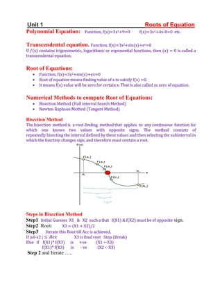
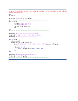
![Q1 Find the root of f x excos x ‐1.2 . Newton Raphson Method.
Acc 0.001.
Given
f x excos x ‐1.2 Function
f ’ x ex cos x ‐sin x Tangent or Slope or Derivative
Solution
Initial Guess
X1 1 And | f X1 | 0.2687 | f ’ X1 | 0.8187
Since | f ’ X1 | | f X1 | Initial Guess is Correct
Step 1 Root
′
Step2 If |x1-x2 | X2 is final root Stop
Else X1 ←X2 and goto Step 1
Result table
‐‐‐‐‐‐‐‐‐‐‐‐‐‐‐‐‐‐‐‐‐‐‐‐‐‐‐‐‐‐‐‐‐‐‐‐‐‐‐‐‐‐‐‐‐‐‐‐‐‐‐‐‐‐‐‐‐‐‐‐‐‐‐‐‐‐‐‐‐‐‐‐‐‐‐‐‐‐‐‐‐‐‐‐‐‐‐‐‐‐‐‐‐‐
I x1 f x1 fd x1 x2 |x1‐x2 |
‐‐‐‐‐‐‐‐‐‐‐‐‐‐‐‐‐‐‐‐‐‐‐‐‐‐‐‐‐‐‐‐‐‐‐‐‐‐‐‐‐‐‐‐‐‐‐‐‐‐‐‐‐‐‐‐‐‐‐‐‐‐‐‐‐‐‐‐‐‐‐‐‐‐‐‐‐‐‐‐‐‐‐‐‐‐‐‐‐‐‐‐‐‐
1 1. 0.2687 ‐0.8187 1.3282 0.3282
2 1.3282 ‐0.2934 ‐2.7571 1.2218 0.1064
3 1.2218 ‐0.0397 ‐2.0284 1.2023 0.0196
4 1.2023 ‐0.0012 ‐1.9054 1.2016 0.0006
‐‐‐‐‐‐‐‐‐‐‐‐‐‐‐‐‐‐‐‐‐‐‐‐‐‐‐‐‐‐‐‐‐‐‐‐‐‐‐‐‐‐‐‐‐‐‐‐‐‐‐‐‐‐‐‐‐‐‐‐‐‐‐‐‐‐‐‐‐‐‐‐‐‐‐‐‐‐‐‐‐‐‐‐‐‐‐‐‐‐‐‐‐‐
As |x1-x2 | .
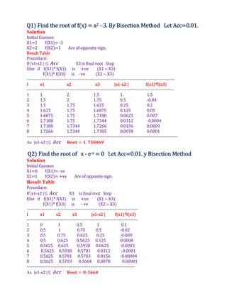
Q1* Find the root of f x excos x ‐1.2 . Newton Raphson Method.
Acc 0.001. Initial Guess is x1 2
| f ’ X1 | | f X1 | ]
Means no need to check](https://image.slidesharecdn.com/1-230606051135-727797a4/85/1-pdf-9-320.jpg)


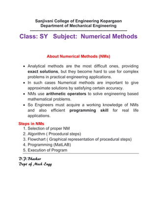
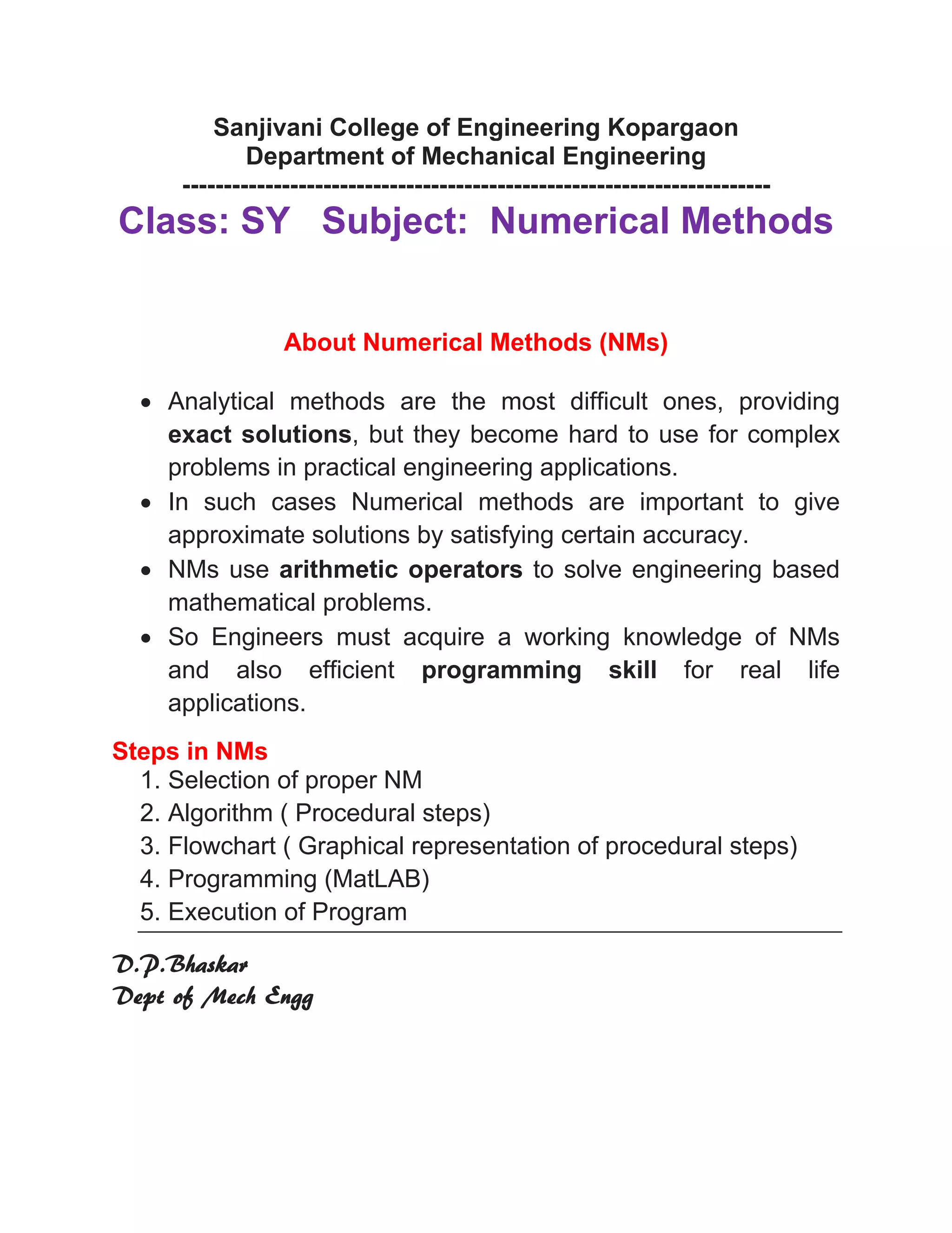
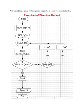
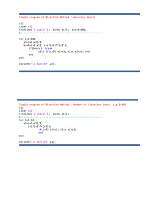
This document discusses numerical methods for solving engineering problems. It introduces numerical methods as ways to find approximate solutions to complex problems that cannot be solved analytically. Bisection and Newton-Raphson methods are described for finding roots of equations. Examples are provided to demonstrate applying the bisection method to find roots of polynomial and transcendental equations. The Newton-Raphson method is also demonstrated for finding roots. Flowcharts and MATLAB programs for implementing the methods are included.


![CH-2_5 ROOTS_OF_NON_LINEAR_EQ [Compatibility Mode].pdf](https://cdn.slidesharecdn.com/ss_thumbnails/ch-25rootsofnonlineareqcompatibilitymode-260123171244-4215d39d-thumbnail.jpg?width=640&height=640&fit=bounds)