Downloaded 650 times
![References
Rao, K.S., Year. Numerical Methods for Scientists and
Engineers. 2nd ed. Delhi: Prentice-Hall of India.
Yousef Sadd and , Henk A. van der Vorst, Iterative Solution of
Linear Systems in the 20th Century [pdf]. Available at: <www-
users.cs.umn.edu/~saad/PDF/umsi-99-152.pdf> Accessed [12th
July 2012]
Relaxation Methods for Iterative Solution to Linear Systems of
Equations Gerald Recktenwald Portland State University
Mechanical Engineering Department
Scientic Computing II Relaxation MethodsMichael Bader
Summer term 2012](https://image.slidesharecdn.com/relaxationmethod-130624231244-phpapp01/75/Relaxation-method-25-2048.jpg)


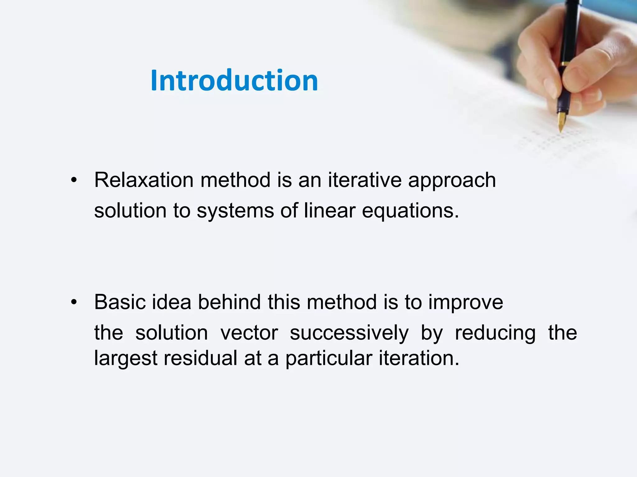
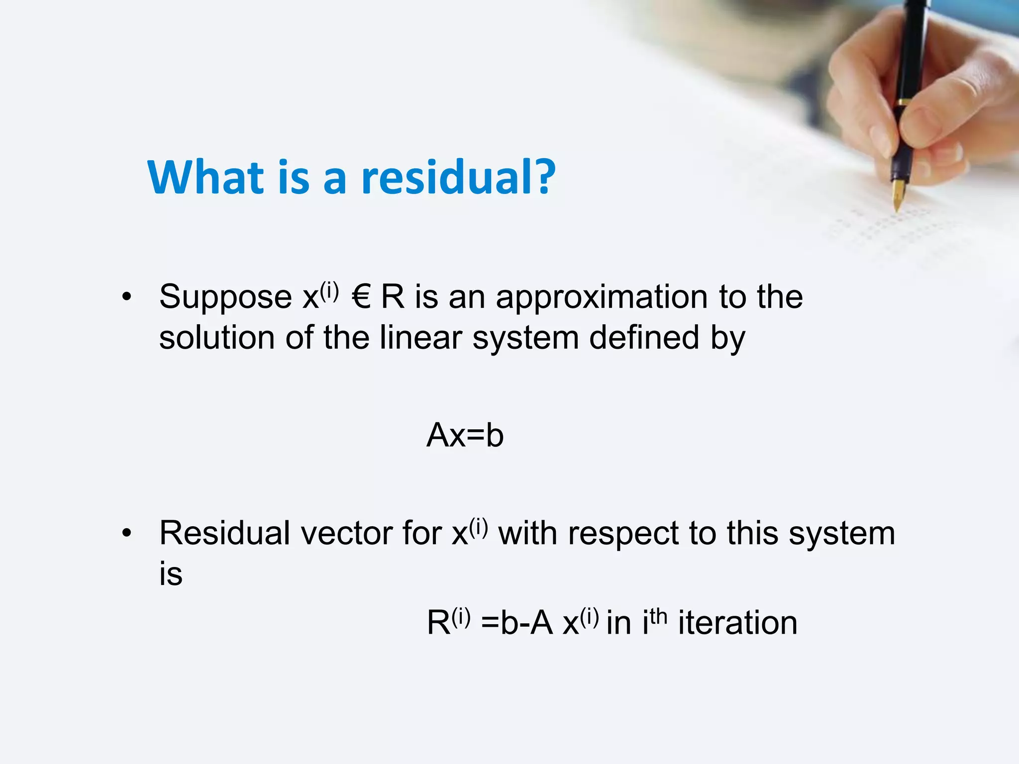
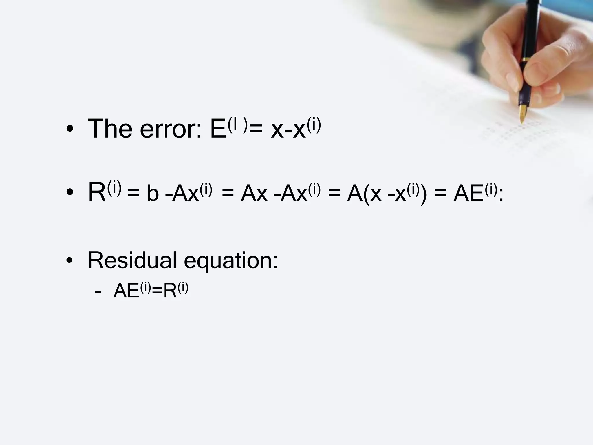
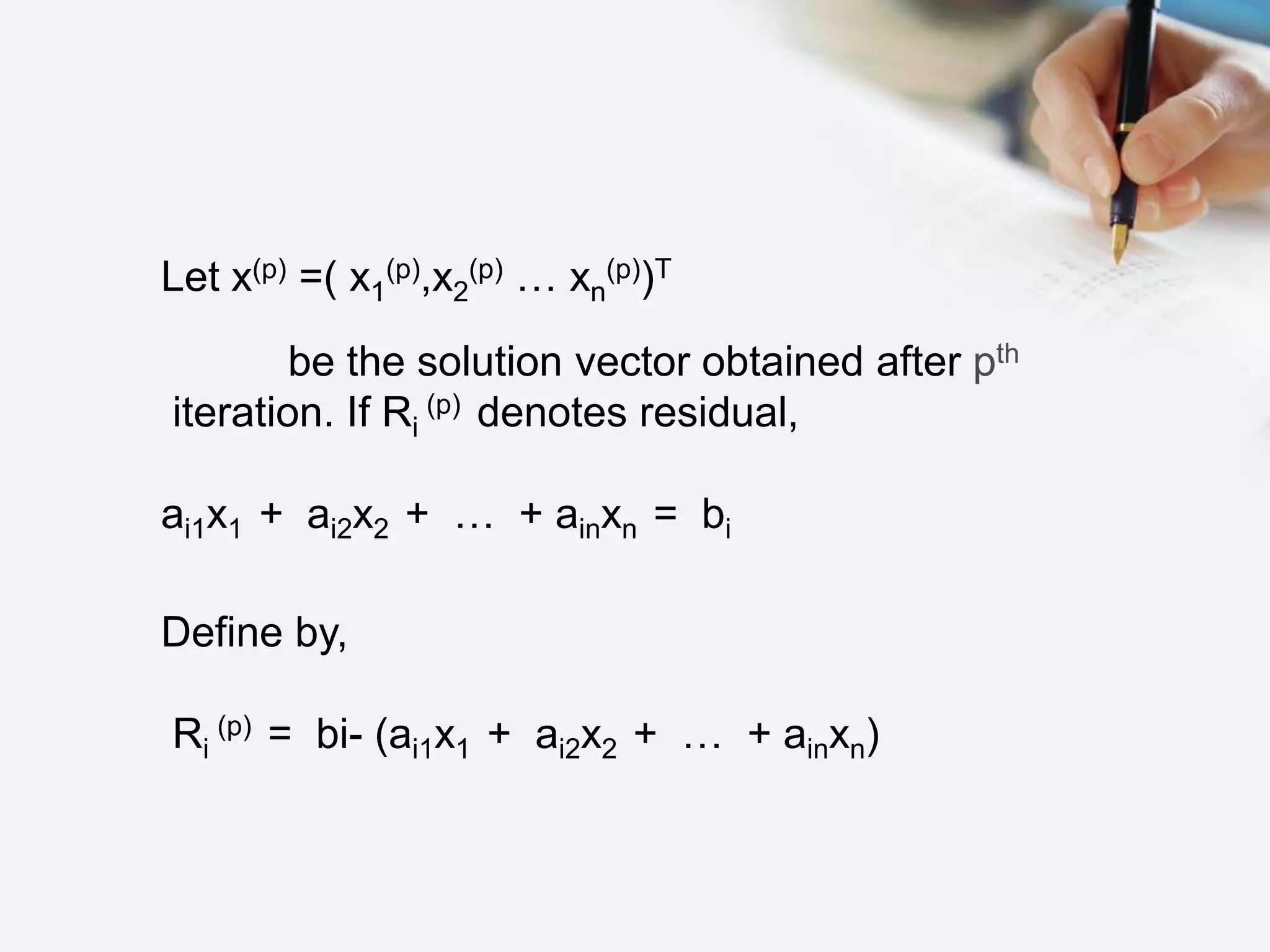
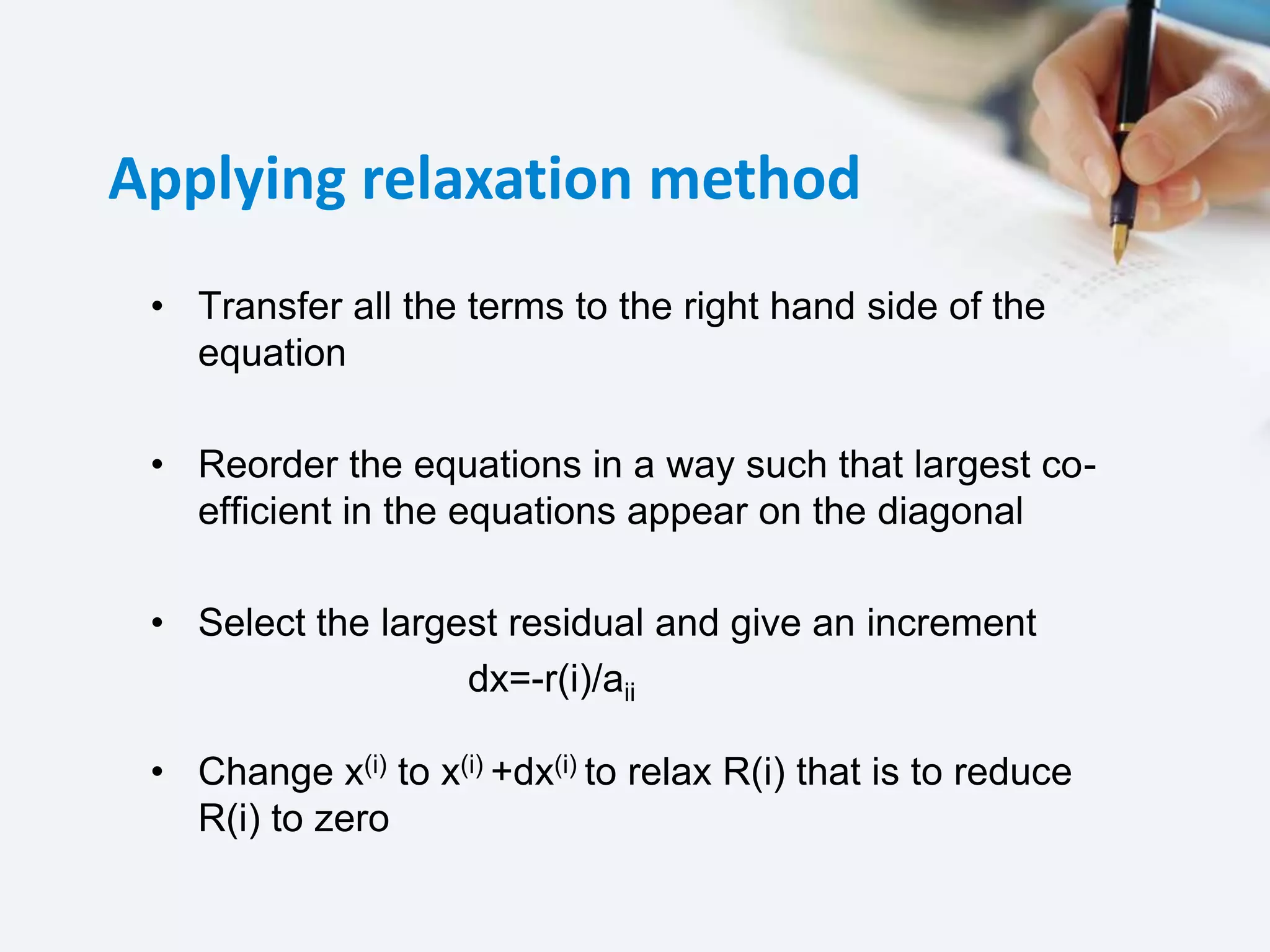
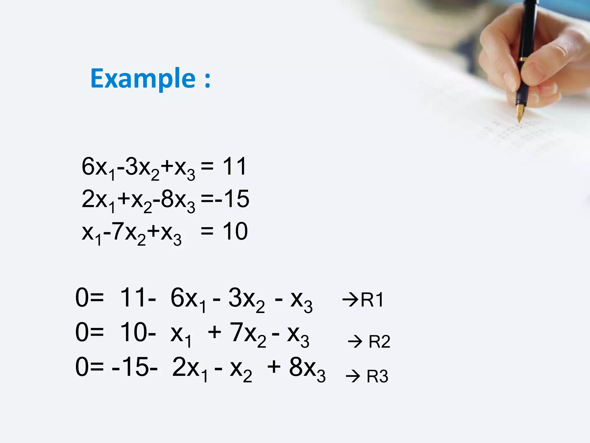
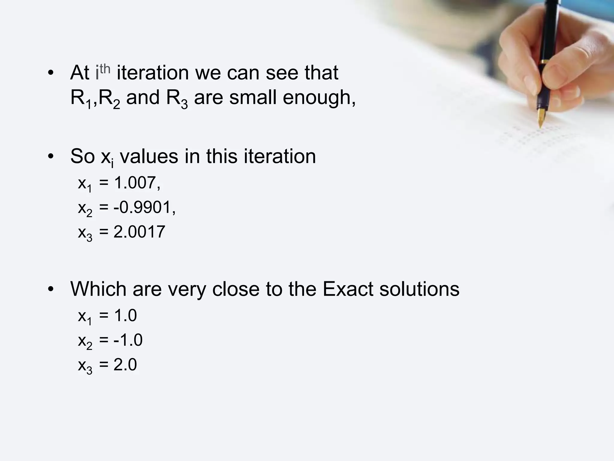
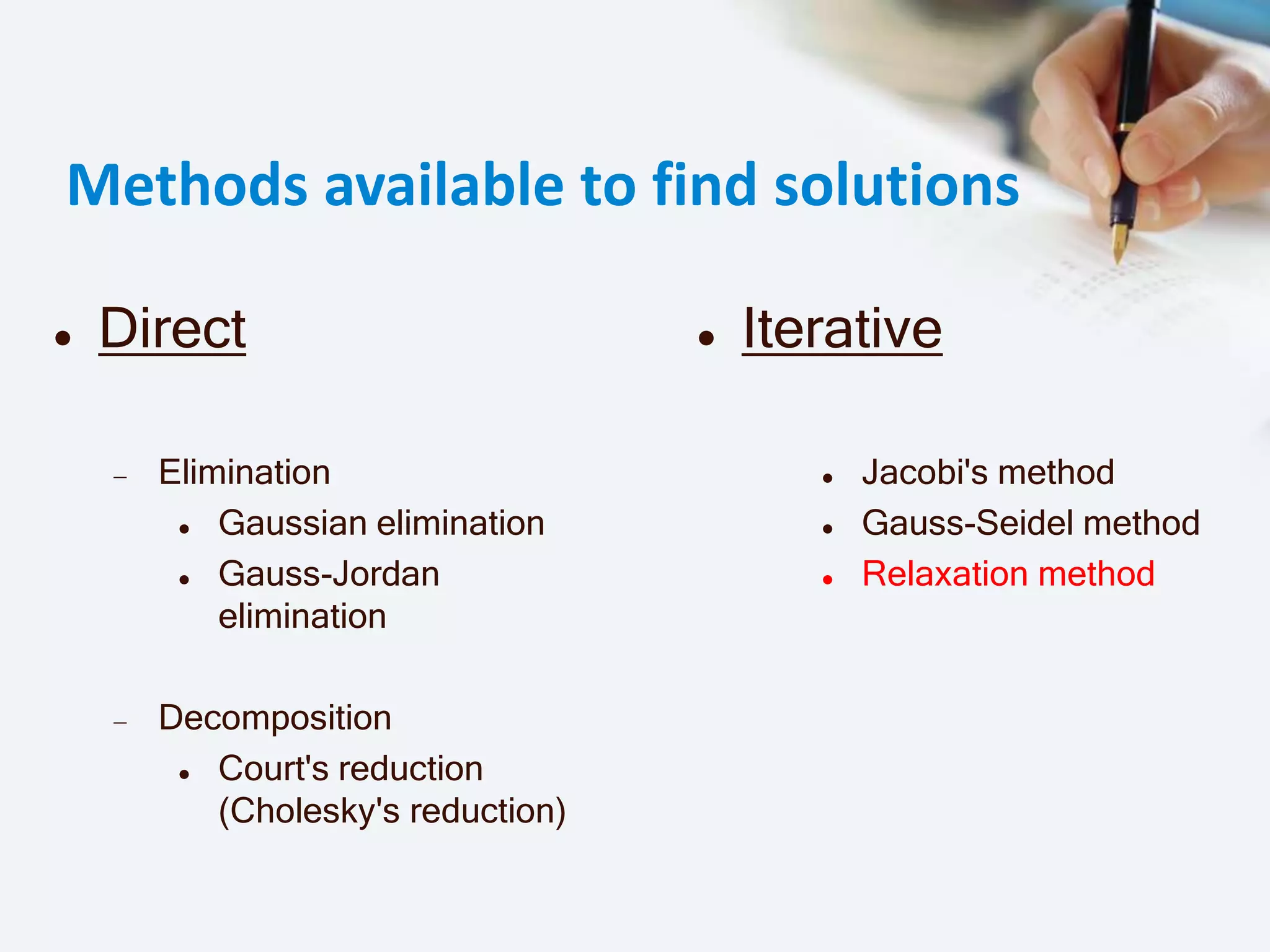
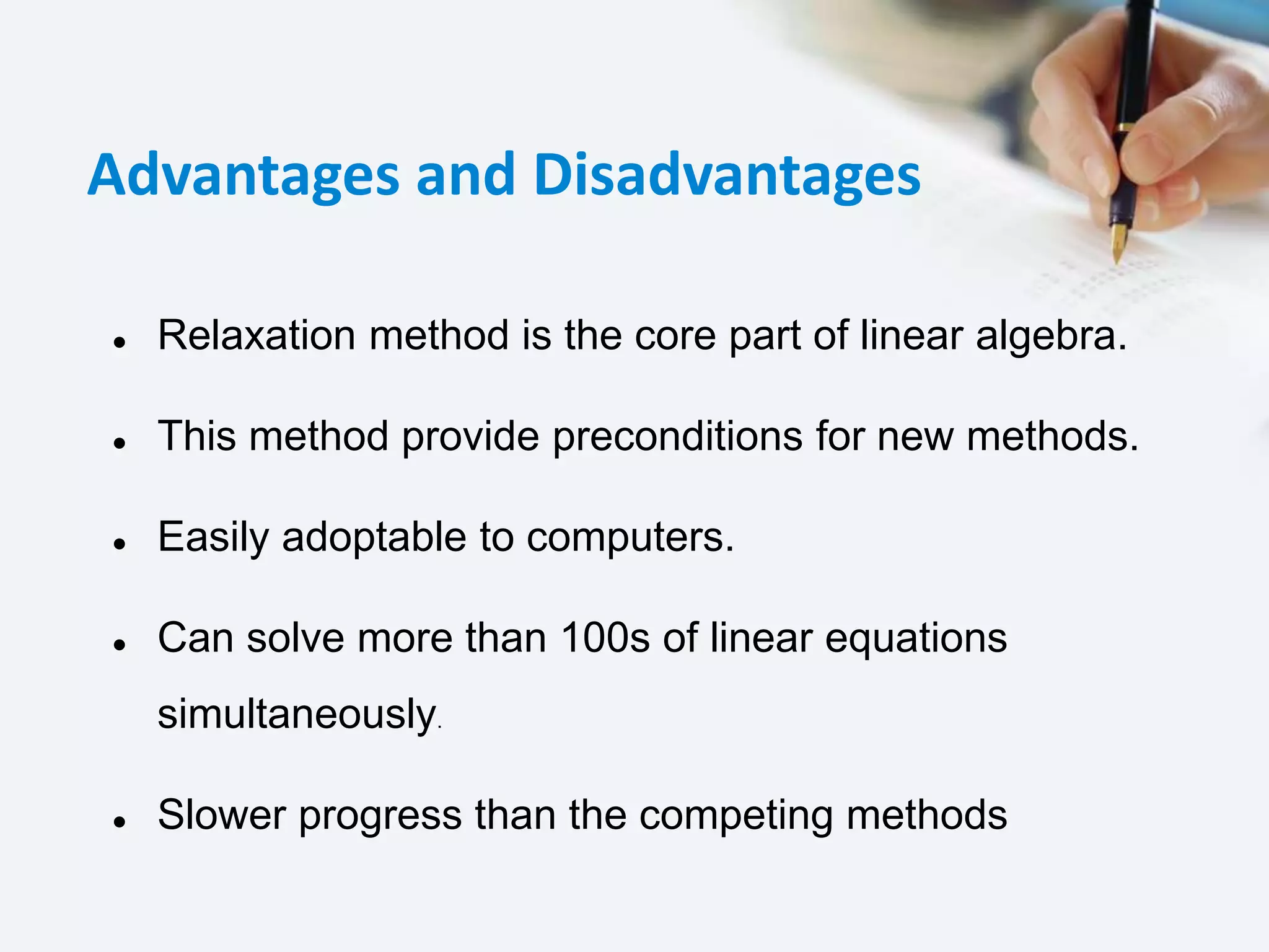
The relaxation method is an iterative technique used to solve systems of linear equations by successively improving the solution vector to minimize the residual error. It involves calculating the residual vector and adjusting the approximation to reduce this residual to zero through a series of iterations. Although it is a fundamental component of linear algebra with applications in various fields, the relaxation method is typically slower than other solution methods and serves more as a preconditioning technique.