This document discusses numerical methods for finding the roots of nonlinear equations. It covers the bisection method, Newton-Raphson method, and their applications. The bisection method uses binary search to bracket the root within intervals that are repeatedly bisected until a solution is found. The Newton-Raphson method approximates the function as a linear equation to rapidly converge on roots. Examples and real-world applications are provided for both methods.

2. 
 Introduction
 Various numerical methods
 Examples
 Real life use
 references
Index

3. 
 Equations that can be cast in the form of a
polynomial are referred to as algebraic equations.
Equations involving more complicated terms, such
as trigonometric, hyperbolic, exponential, or
logarithmic functions are referred to as
transcendental equations. The methods presented in
this section are numerical methods that can be
applied to the solution of such equations, to which
we will refer, in general, as non-linear equations. In
general, we will we searching for one, or more,
solutions to the equation, f(x) = 0.
3
Introduction

4. 
 Bisection method
 Newton – Raph son method
 Secant method
 False position method, etc
4
Various numerical
methods find the roots

5. 
The History of the Bisection Method
 Although there is little concrete knowledge of the
development the bisection method, we can infer that
it was developed a short while after the Intermediate
Value Theorem was first proven by Bernard Bolzano
in 1817 (Edwards 1979). It appears that it was used
as a proof of an intermediate theorem to the general
proof Bolzano was developing for the Intermediate
Value Theorem
5
Bisection method

6. 6

7. 
 If a function f(x) is continuous and there is a point a
that is negative and a point b that is positive then
there is a point c between (a,b) that equal zero. An
interval is always chosen in [a,b] which includes the
root somewhere within. That interval [a,b] is then cut
in half, and the half that contains the root is then
chosen. That new interval is then cut in half once
again, and the half that contains the root is chosen
once again. The bisection method repeats these steps
numerous times until the approximation is within a
certain degree
7
procedure

8. 8
Example 1
Consider finding the root of f(x) = x2 - 3. Let εstep = 0.01, εabs = 0.01 and start with the
interval [1, 2].
Table 1. Bisection method applied to f(x) = x2 - 3.
a b f(a) f(b)
c = (a +
b)/2
f(c) Update
new b −
a
1.0 2.0 -2.0 1.0 1.5 -0.75 a = c 0.5
1.5 2.0 -0.75 1.0 1.75 0.062 b = c 0.25
1.5 1.75 -0.75 0.0625 1.625 -0.359 a = c 0.125
1.625 1.75 -0.3594 0.0625 1.6875 -0.1523 a = c 0.0625
1.6875 1.75 -0.1523 0.0625 1.7188 -0.0457 a = c 0.0313
1.7188 1.75 -0.0457 0.0625 1.7344 0.0081 b = c 0.0156
1.71988
/td>
1.7344 -0.0457 0.0081 1.7266 -0.0189 a = c 0.0078

9. 9
2.
2. Find the root of x4-x-10 = 0
The graph of this equation is given in the figure.
Let a = 1.5 and b = 2
Iteration
No.
a b c f(a) * f(c)
1 1.5 2 1.75 15.264 (+ve)
2 1.75 2 1.875 -1.149 (-ve)
3 1.75 1.875 1.812 2.419 (+ve)
4 1.812 1.875 1.844 0.303 (-ve)
5 1.844 1.875 1.86 -0.027 (-ve)
So one of the roots of x4-x-10 = 0 is approximately 1.86

10. 
 One of the biggest advantages to the bisection
method is that it never diverges. Error also
decreases with each iteration. Therefore, as the
interval keeps splitting, the approximation gets closer
and closer to the desired root
10
advantages

11. 
 The biggest disadvantage of the bisection method is that
it converges slower than other methods and it cannot
depict multiple roots. Furthermore, if two roots lie close to
each other then the bisection method makes it difficult to
find both roots simultaneously. In the specific case of
f(x)=x2, the bisection method fails to converge on the root
(0,0). If a point a is chosen to the left of the zero and the
same point is taken to the right of the zero then the root
will not be found.
11
Disadvantages

12. 
 Shot Detection in Video Content for Digital Video Library -
The study presented the usage of bisection method for shot
detection in video content for the Digital Video Library (DVL).
DVL is a networked Internet application allowing for storage,
searching, cataloguing, browsing, retrieval, searching and uni-
casting video sequences. The browsing functionality can be
significantly facilitated by a fast shot detection process.
Experiments show that usage of the bisection method, allows
for accelerating shot detection about 3÷150 times (related to the
shot density). At the end of the paper two possible networked
applications are presented: a medical DVL developed for
elearning purposes and a hypothetical networked news
application
12
Real-Life Applications

13. 13
 Locating and computing periodic orbits in molecular
systems - The Characteristic Bisection Method for finding
the roots of non-linear algebraic and/or transcendental
equations is applied to Li NC/Li CN molecular system to
locate periodic orbits and to construct the
continuation/bifurcation diagram of the bend mode
family. The algorithm is based on the Characteristic Poly
hidra which define a domain in phase space where the
topological degree is not zero. The results are compared
with previous calculations obtained by the Newton
Multiple Shooting algorithm. The Characteristic Bisection
Method not only reproduces the old results, but also,
locates new symmetric and asymmetric families of
periodic orbits of high multiplicity.
 Bisection method for determining an adequate
population size

14. 14

15. 
 The name "Newton's method" is derived from Isaac Newton's
description of a special case of the method in De analysi per
aequationes numero terminorum infinitas (written in 1669,
published in 1711 by William Jones) and in De metodis
fluxionum et serierum infinitarum (written in 1671, translated
and published as Method of Fluxions in 1736 by John Colson).
However, his method differs substantially from the modern
method given above: Newton applies the method only to
polynomials.
15
History

16. 16
• He does not compute the successive approximations x_n, but computes a
sequence of polynomials, and only at the end arrives at an approximation for
the root x. Finally, Newton views the method as purely algebraic and makes
no mention of the connection with calculus. Newton may have derived his
method from a similar but less precise method by Vieta. The essence of
Vieta's method can be found in the work of the Persian mathematician
Sharaf al-Din al-Tusi, while his successor Jamshīd al-Kāshī used a form of
Newton's method to solve x^P - N = 0 to find roots of N (Ypma 1995).
• Newton's method was first published in 1685 in A Treatise of Algebra both
Historical and Practical by John Wallis. In 1690, Joseph Raphson published a
simplified description in Analysis aequationum universalis. Raphson again
viewed Newton's method purely as an algebraic method and restricted its
use to polynomials, but he describes the method in terms of the successive
approximations xn instead of the more complicated sequence of
polynomials used by Newton. Finally, in 1740, Thomas Simpson described
Newton's method as an iterative method for solving general nonlinear
equations using calculus, essentially giving the description above. In the
same publication, Simpson also gives the generalization to systems of two
equations and notes that Newton's method can be used for solving
optimization problems by setting the gradient to zero.

17. 17
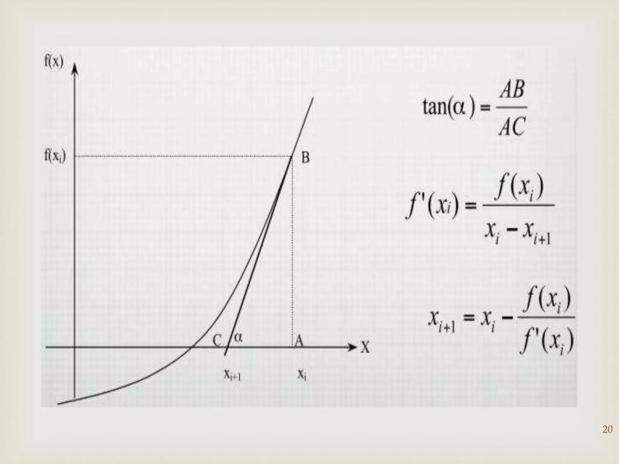
Unlike the earlier methods, this method requires only one
appropriate starting point as an initial assumption of the root of
the function At a tangent to is drawn.
Equation of this tangent is given by
• The point of intersection, say , of this tangent with x-axis (y = 0)
is taken to be the next approximation to the root of f(x) = 0. So on
substituting y = 0 in the tangent equation we get

18. )( 00 xfy  and
10
0
0
xx
y
x
dx
dy

atWe have and we need to find .
1x
Then,
10
0
0
/ )(
)(
xx
xf
xf


Rearranging:
)(
)(
0
/
0
10
xf
xf
xx 
)(
)(
0
/
0
01
xf
xf
xx 
Using and in the formula isn’t very
convenient, so, since we have)(xfy 
0at x
dx
dy
0y
)( 0
/
10
0
0 xf
xx
y
x
dx
dy


at

19. )(
)(
0
/
0
01
xf
xf
xx So,
We just need to alter the subscripts to find : 2x
)(
)(
1
/
1
12
xf
xf
xx 
Generalising gives
)(
)(
/1
n
n
nn
xf
xf
xx 
We don’t need a diagram to use this formula but we
must know how to differentiate . )(xf
Convergence is often very fast.

20. 20

21. 21
We will use the Newton-Raphson method to find the positive root of the equation sinx = x2,
correct to 3D.
It will be convenient to use the method of false position to obtain an initial approximation.
Tabulating, one finds
With numbers displayed to 4D, we see that there is a root in the interval 0.75 < x < 1
at approximately
Example: 1

22. 22
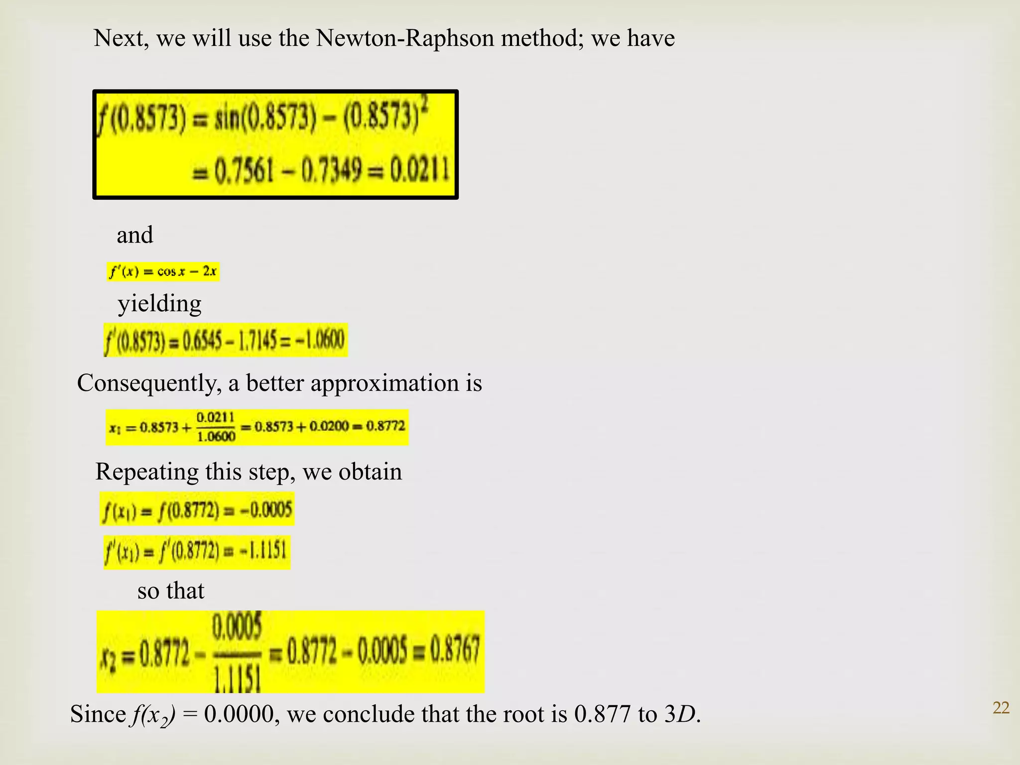
Next, we will use the Newton-Raphson method; we have
and
yielding
Consequently, a better approximation is
Repeating this step, we obtain
so that
Since f(x2) = 0.0000, we conclude that the root is 0.877 to 3D.

23. 
 The method is very expensive - It needs the function
evaluation and then the derivative evaluation.
 If the tangent is parallel or nearly parallel to the x-axis,
then the method does not converge.
 Usually Newton method is expected to converge only
near the solution.
 The advantage of the method is its order of convergence
is quadratic.
 Convergence rate is one of the fastest when it does
converge.
23
Advantages and
Disadvantages

24. 
 Applying NR to the system of equations we find that at
iteration k+1:
 all the coefficients of KCL, KVL and of BCE of the linear
elements remain unchanged with respect to iteration k
 Nonlinear elements are represented by a linearization of
BCE around iteration k
 This system of equations can be interpreted as the STA of
a linear circuit (companion network) whose elements are
specified by the linearized BCE.
 APPLICATION OF NEWTON RAPHSON METHOD TO
A FINITE BARRIER QUANTUM WELL (FBQW)
SYSTEM
Real life uses

25. 
25
References
• http://www2.lv.psu.edu/ojj/courses/cmpsc-
201/numerical/bisection.html
• http://en.wikipedia.org/wiki/Bisection_method#Pseudo-
code
• Bisection Method, Autar Kaw and Jai
Paul, http://numericalmethods.eng.usf.edu
• http://newtons.wikia.com/wiki/NewtonRaphson_Wiki

26. 26