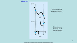
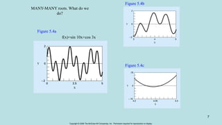
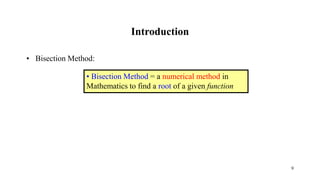
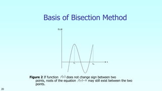
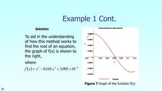
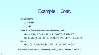
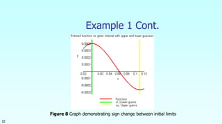
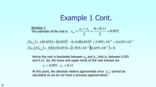
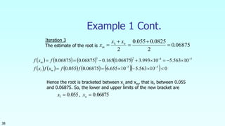
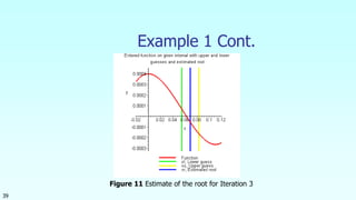
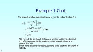
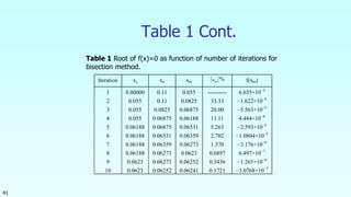
This document discusses the bisection method for finding roots of equations. It begins by introducing the bisection method and explaining that it uses an initial interval that brackets a root to successively narrow down the interval containing the root. It then provides the steps of the bisection method algorithm. Finally, it includes an example of applying the bisection method to find the depth at which a floating ball is submerged. Over 10 iterations, the method converges on a root of 0.06252 within the specified error tolerance.


![A Mathematical Property
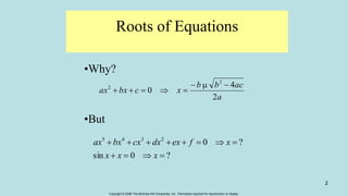
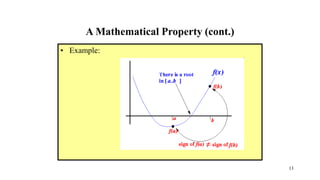
• Well-known Mathematical Property:
• If a function f(x) is continuous on the interval [a..b] and
sign of f(a) ≠ sign of f(b), then
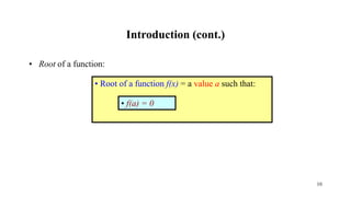
• There is a value c ∈ [a..b] such that: f(c) =
0 I.e., there is a root c in the interval [a..b]
12](https://image.slidesharecdn.com/nm-lec2-170909205626/85/Numerical-Method-2-12-320.jpg)
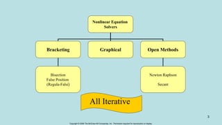
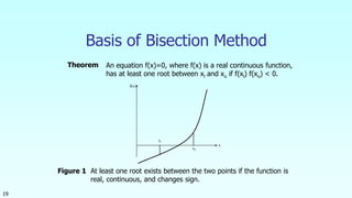
![The Bisection Method
• The Bisection Method is a successive approximation method
that narrows down an interval that contains a root of the
function f(x)
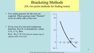
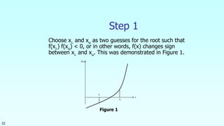
• The Bisection Method is given an initial interval [a..b] that
contains a root (We can use the property sign of f(a) ≠ sign of
f(b) to find such an initial interval)
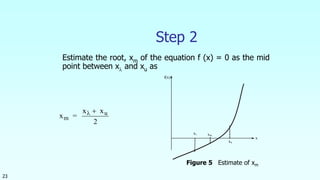
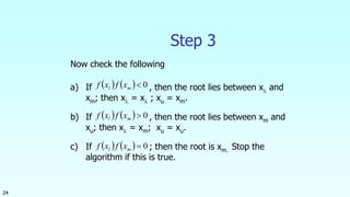
• The Bisection Method will cut the interval into 2 halves and
check which half interval contains a root of the function
• The Bisection Method will keep cut the interval in halves until
the resulting interval is extremely small
The root is then approximately equal to any value in the final
(very small) interval.
14](https://image.slidesharecdn.com/nm-lec2-170909205626/85/Numerical-Method-2-14-320.jpg)
![The Bisection Method (cont.)
• Example:
• Suppose the interval [a..b] is as follows:
15](https://image.slidesharecdn.com/nm-lec2-170909205626/85/Numerical-Method-2-15-320.jpg)
![The Bisection Method (cont.)
• We cut the interval [a..b] in the middle: m = (a+b)/2
16](https://image.slidesharecdn.com/nm-lec2-170909205626/85/Numerical-Method-2-16-320.jpg)
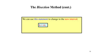
![The Bisection Method (cont.)
• Because sign of f(m) ≠ sign of f(a) , we proceed with the
search in the new interval [a..b]:
17](https://image.slidesharecdn.com/nm-lec2-170909205626/85/Numerical-Method-2-17-320.jpg)


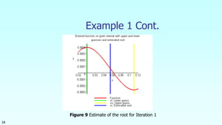
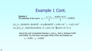
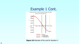
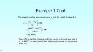


![CH-2_5 ROOTS_OF_NON_LINEAR_EQ [Compatibility Mode].pdf](https://cdn.slidesharecdn.com/ss_thumbnails/ch-25rootsofnonlineareqcompatibilitymode-260123171244-4215d39d-thumbnail.jpg?width=640&height=640&fit=bounds)