lecture 2

1. 1
Bisection Method

2. 2
Absolute Error
Given an approximation a of a correct value x, we define
the absolute value of the difference between the two
values to be the absolute error. We will represent the
absolute error by Eabs,
Relative Error
Thus, we define the relative error to be the ratio between the
absolute error and the absolute value of the correct value
and denote it by Erel:

3. 3
Calculating Absolute Error AND Relative Error

4. 4
H.W
Calculate Relative Error of:
Where N is the count rate of the sample, B is the background count
rate, t is the counting time (s), is the probability of gamma decay
(%), f is detector efficiency (%), m is the mass (kg) of the sediment
sample.

5. 5
Basis of Bisection Method
Theorem
x
f(x)
xu
x
An equation f(x)=0, where f(x) is a real continuous
function, has at least one root between xl and xu if f(xl) f(xu)
< 0.
Figure 1 At least one root exists between the two points if the function
is real, continuous, and changes sign.

6. x
f(x)
xu
x
6
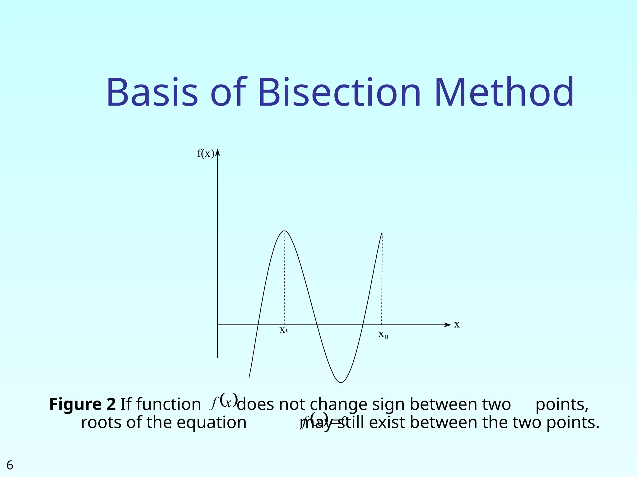
Basis of Bisection Method
Figure 2 If function does not change sign between two points,
roots of the equation may still exist between the two points.
 
x
f
  0

x
f

7. x
f(x)
xu
x
7
Basis of Bisection Method
Figure 3 If the function does not change sign between two
points, there may not be any roots for the equation between
the two points.
x
f(x)
xu
x
 
x
f
  0

x
f

8. x
f(x)
xu
x
8
Basis of Bisection Method
Figure 4 If the function changes sign between two points,
more than one root for the equation may exist between the
two points.
 
x
f
  0

x
f

9. 9
Algorithm for Bisection
Method

10. http://numericalmethods.eng.usf.edu
10

11. 11
Step 1
Choose xl
and xu
as two guesses for the root such
that f(xl
) f(xu
) < 0, or in other words, f(x) changes sign
between xl
and xu
. This was demonstrated in Figure
1.
x
f(x)
xu
x
Figure 1

12. x
f(x)
xu
x
xm
12
Step 2
Estimate the root, xm
of the equation f (x) = 0 as the
mid point between xl
and xu
as
x
x
m =
xu
 
2
Figure 5 Estimate of xm

13. 13
Step 3
Now check the following
a) If , then the root lies between xl
and xm
;
then xl
= xl
; xu
= xm
.
b) If , then the root lies between xm
and
xu
; then xl
= xm
; xu
= xu
.
c) If ; then the root is xm.
Stop the
algorithm if this is true.
    0

m
l x
f
x
f
    0

m
l x
f
x
f
    0

m
l x
f
x
f

14. 14
Step 4
x
x
m =
xu
 
2
100



 new
m
old
m
new
a
x
x
xm
root
of
estimate
current

new
m
x
root
of
estimate
previous

old
m
x
Find the new estimate of the root
Find the absolute relative approximate error
where

15. 15
Step 5
Is ?
Yes
No
Go to Step 2 using
new upper and lower
guesses.
Stop the algorithm
Compare the absolute relative approximate error
with the pre-specified error tolerance .
a

s

s
a 

Note one should also check whether the number of
iterations is more than the maximum number of
iterations allowed. If so, one needs to terminate the
algorithm and notify the user about it.

16. http://numericalmethods.eng.usf.edu
16

17. 17
Example 1
You are working for ‘DOWN THE TOILET COMPANY’
that makes floats for ABC commodes. The floating
ball has a specific gravity of 0.6 and has a radius of
5.5 cm. You are asked to find the depth to which the
ball is submerged when floating in water.
Figure 6 Diagram of the floating ball

18. 18
Example 1 Cont.
The equation that gives the depth x to which the ball
is submerged under water is given by
a) Use the bisection method of finding roots of
equations to find the depth x to which the ball is
submerged under water. Conduct three iterations to
estimate the root of the above equation.
b) Find the absolute relative approximate error at the
end of each iteration, and the number of significant
digits at least correct at the end of each iteration.
0
10
993
.
3
165
.
0 4
2
3



 
x
x

19. 19
Example 1 Cont.
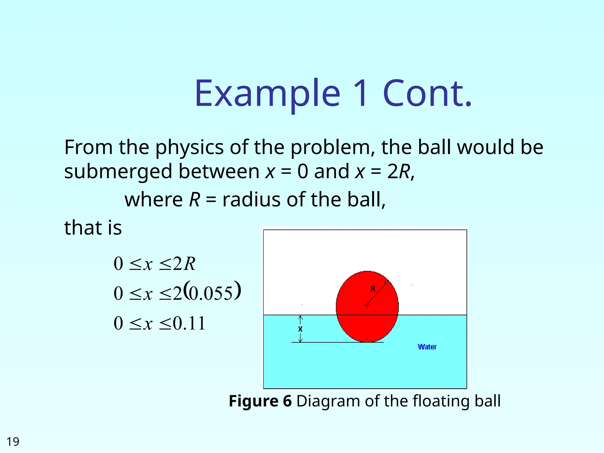
From the physics of the problem, the ball would be
submerged between x = 0 and x = 2R,
where R = radius of the ball,
that is
 
11
.
0
0
055
.
0
2
0
2
0






x
x
R
x
Figure 6 Diagram of the floating ball

20. To aid in the
understanding of how this
method works to find the
root of an equation, the
graph of f(x) is shown to
the right,
where
20
Example 1 Cont.
 0
10
4.2
03
.0 6
2
3



 
x
x
x
x
f
  4
2
3
10
993
3
165
0 -
.
x
.
x
x
f 



Figure 7 Graph of the function f(x)
Solution

21. 21
Example 1 Cont.
Let us assume
11
.
0
00
.
0


u
x
x
Check if the function changes sign between xl
and
xu .        
        4
4
2
3
4
4
2
3
10
662
.
2
10
993
.
3
11
.
0
165
.
0
11
.
0
11
.
0
10
993
.
3
10
993
.
3
0
165
.
0
0
0



















f
x
f
f
x
f
u
l
Hence
           0
10
662
.
2
10
993
.
3
11
.
0
0 4
4





 

f
f
x
f
x
f u
l
So there is at least on root between xl
and xu,
that is between 0 and
0.11

22. 22
Example 1 Cont.
Figure 8 Graph demonstrating sign change between initial
limits

23. 23
Example 1 Cont.
055
.
0
2
11
.
0
0
2




 u
m
x
x
x 
       
           0
10
655
.
6
10
993
.
3
055
.
0
0
10
655
.
6
10
993
.
3
055
.
0
165
.
0
055
.
0
055
.
0
5
4
5
4
2
3
















f
f
x
f
x
f
f
x
f
m
l
m
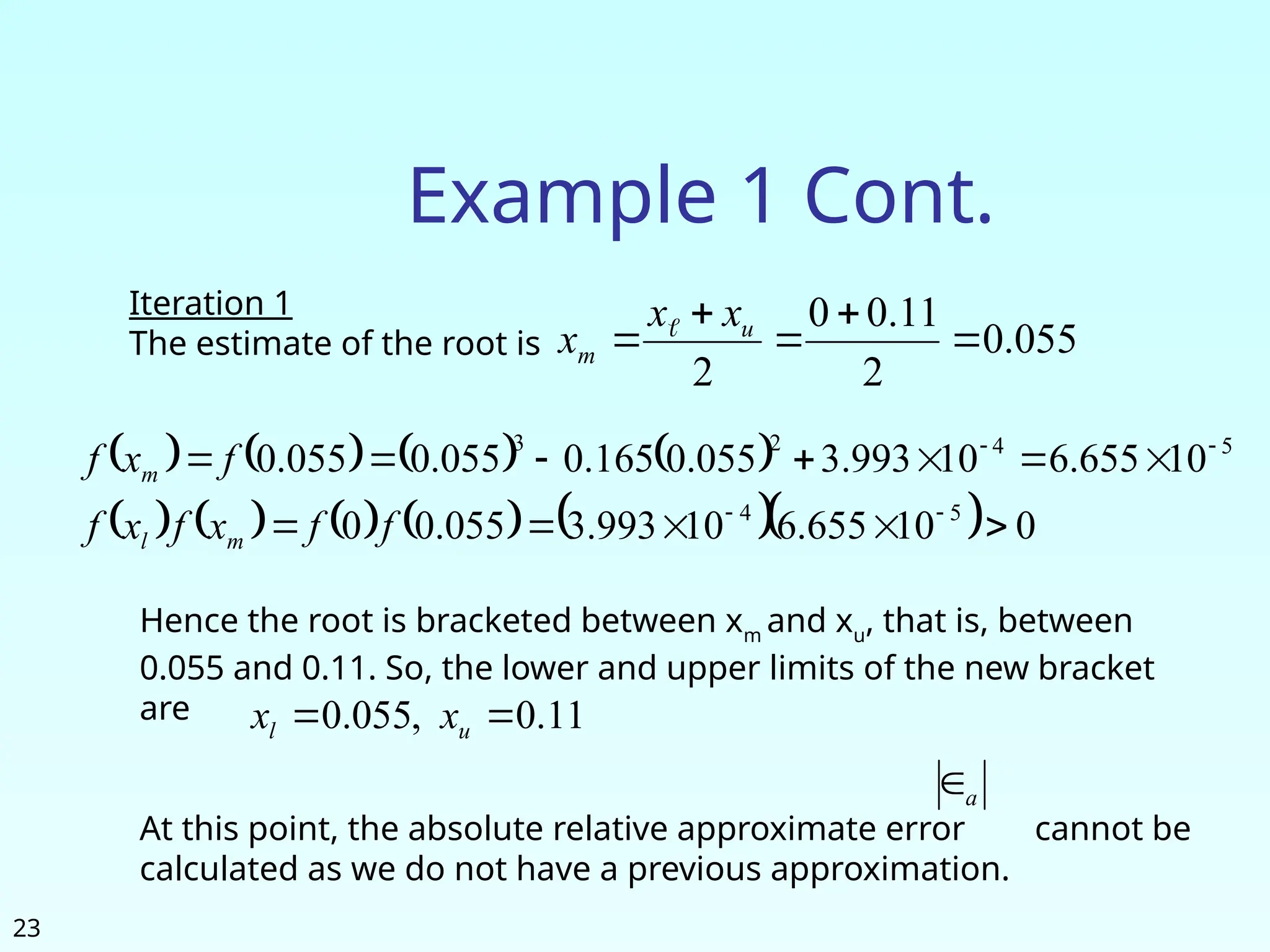
Iteration 1
The estimate of the root is
Hence the root is bracketed between xm
and xu
, that is, between
0.055 and 0.11. So, the lower and upper limits of the new bracket
are
At this point, the absolute relative approximate error cannot be
calculated as we do not have a previous approximation.
11
.
0
,
055
.
0 
 u
l x
x
a


24. 24
Example 1 Cont.
Figure 9 Estimate of the root for Iteration 1

25. 25
Example 1 Cont.
0825
.
0
2
11
.
0
055
.
0
2




 u
m
x
x
x 
       
         0
10
655
.
6
10
622
.
1
)
0825
.
0
(
055
.
0
10
622
.
1
10
993
.
3
0825
.
0
165
.
0
0825
.
0
0825
.
0
5
4
4
4
2
3


















f
f
x
f
x
f
f
x
f
m
l
m
Iteration 2
The estimate of the root is
Hence the root is bracketed between xl
and xm
, that is, between
0.055 and 0.0825. So, the lower and upper limits of the new bracket
are 0825
.
0
,
055
.
0 
 u
l x
x

26. 26
Example 1 Cont.
Figure 10 Estimate of the root for Iteration 2

27. 27
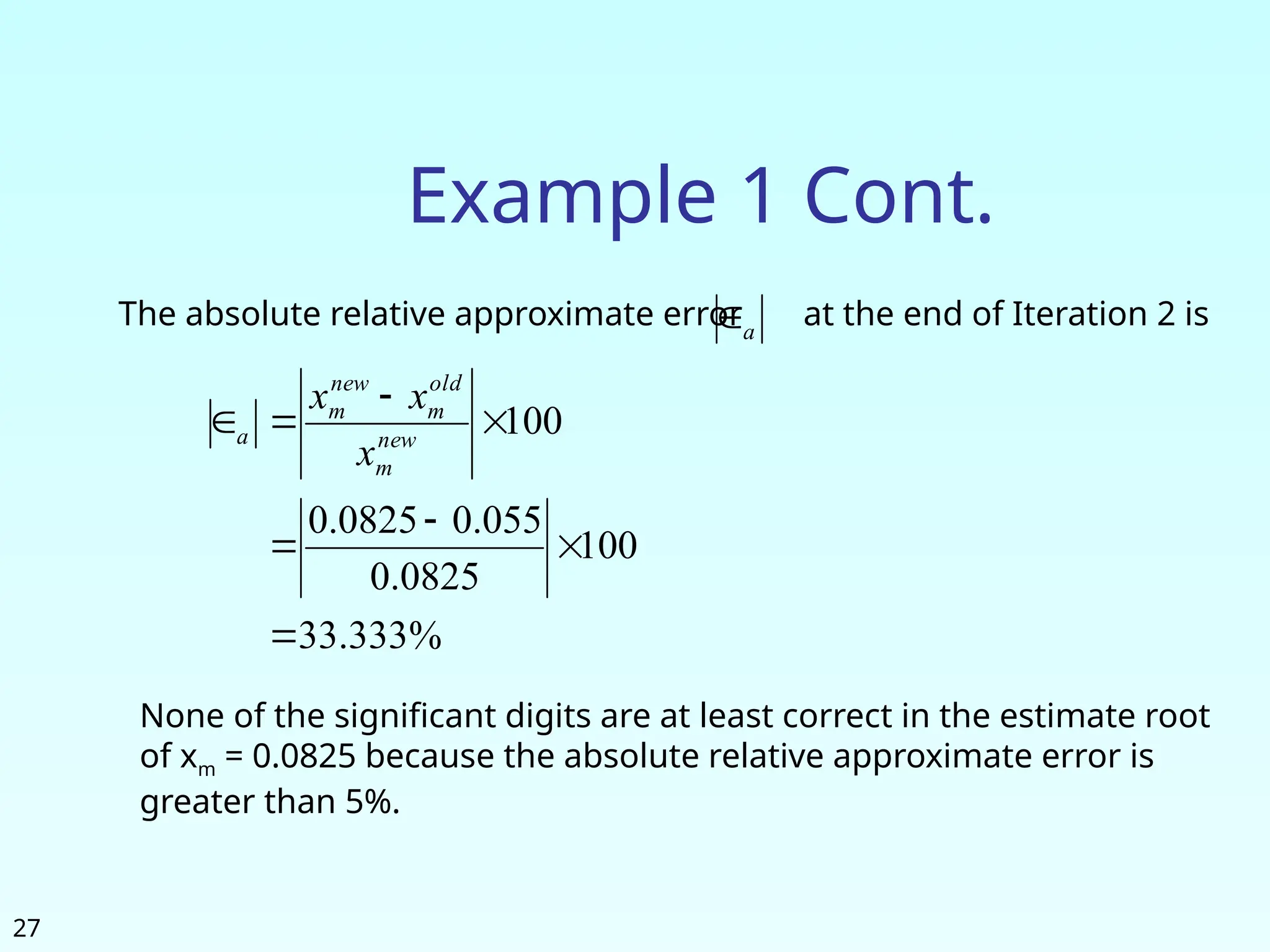
Example 1 Cont.
The absolute relative approximate error at the end of Iteration 2 is
a

%
333
.
33
100
0825
.
0
055
.
0
0825
.
0
100







 new
m
old
m
new
m
a
x
x
x
None of the significant digits are at least correct in the estimate root
of xm = 0.0825 because the absolute relative approximate error is
greater than 5%.

28. 28
Example 1 Cont.
06875
.
0
2
0825
.
0
055
.
0
2




 u
m
x
x
x 
       
           0
10
563
.
5
10
655
.
6
06875
.
0
055
.
0
10
563
.
5
10
993
.
3
06875
.
0
165
.
0
06875
.
0
06875
.
0
5
5
5
4
2
3


















f
f
x
f
x
f
f
x
f
m
l
m
Iteration 3
The estimate of the root is
Hence the root is bracketed between xl
and xm
, that is, between
0.055 and 0.06875. So, the lower and upper limits of the new
bracket are 06875
.
0
,
055
.
0 
 u
l x
x

29. 29
Example 1 Cont.
Figure 11 Estimate of the root for Iteration 3

30. 30
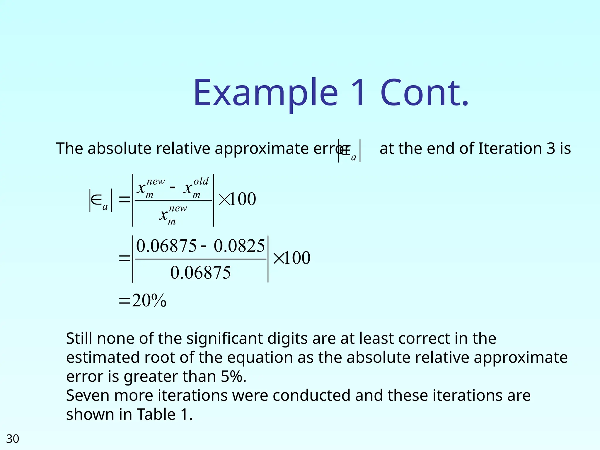
Example 1 Cont.
The absolute relative approximate error at the end of Iteration 3 is
a

%
20
100
06875
.
0
0825
.
0
06875
.
0
100







 new
m
old
m
new
m
a
x
x
x
Still none of the significant digits are at least correct in the
estimated root of the equation as the absolute relative approximate
error is greater than 5%.
Seven more iterations were conducted and these iterations are
shown in Table 1.

31. 31
Table 1 Cont.
Table 1 Root of f(x)=0 as function of number of iterations for
bisection method.
Iteration x xu xm a % f(xm)
1
2
3
4
5
6
7
8
9
10
0.00000
0.055
0.055
0.055
0.06188
0.06188
0.06188
0.06188
0.0623
0.0623
0.11
0.11
0.0825
0.06875
0.06875
0.06531
0.06359
0.06273
0.06273
0.06252
0.055
0.0825
0.06875
0.06188
0.06531
0.06359
0.06273
0.0623
0.06252
0.06241
----------
33.33
20.00
11.11
5.263
2.702
1.370
0.6897
0.3436
0.1721
6.655×10−5
−1.622×10−4
−5.563×10−5
4.484×10−6
−2.593×10−5
−1.0804×10−5
−3.176×10−6
6.497×10−7
−1.265×10−6
−3.0768×10−7

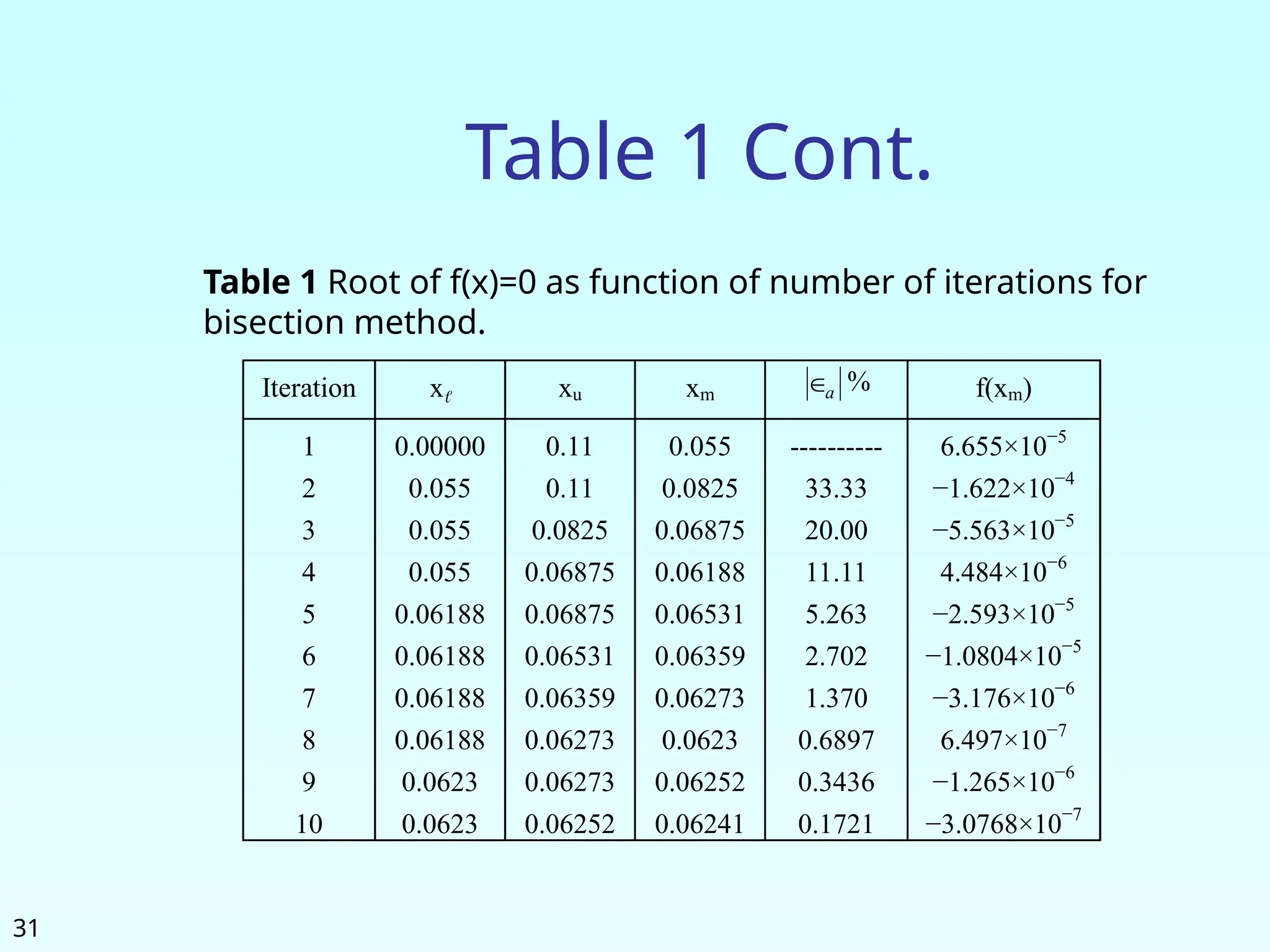
32. 32
Table 1 Cont.
Hence the number of significant digits at least correct is given by
the largest value or m for which
 
  463
.
2
3442
.
0
log
2
2
3442
.
0
log
10
3442
.
0
10
5
.
0
1721
.
0
10
5
.
0
2
2
2














m
m
m
m
m
a
2

m
So
The number of significant digits at least correct in the estimated
root of 0.06241 at the end of the 10th
iteration is 2.

33. 33
Advantages
 Always convergent
 The root bracket gets halved with
each iteration - guaranteed.

34. 34
Drawbacks
 Slow convergence
 If one of the initial guesses is close to
the root, the convergence is slower

35. 35
Drawbacks (continued)
 If a function f(x) is such that it just
touches the x-axis it will be unable to
find the lower and upper guesses.
f(x)
x
  2
x
x
f 