SlideShare a Scribd company logo
1 of 120
Numerical Analysis for Engineers
Roots of equations
Roots of equations
The solution of f(x) is given by the quadratic formula:
The values of x’s are called roots of the function f(x) and they
represent the values of x that make f(x) =0. For this reason roots are
called sometimes zeros of the equation.
Although the quadratic formula is handy for solving f(x), there are
many other functions for which the root can’t be determined so
easily.
For these cases we are going to study Numerical methods that provide
different means to obtain the answer.
Roots of equations
Nonlinear Equation
Solvers
Bracketing Graphical Open Methods
Bisection
False Position
(Regula-Falsi)
Newton Raphson
Secant
Graphical methods
• Make a plot of f(x) and see when f(x) crosses
the x axis.
• This point represents the value of x for which
f(x)=0
Example
• Use the graphical approach to determine the
root of f(x)=x-14.5
x F(x)
4 -10.5
8 -6.5
12 -2.5
16 1.5
20 5.5 -12
-10
-8
-6
-4
-2
0
2
4
6
8
0 2 4 6 8 10 12 14 16 18 20 22
Eng. Muhannad Al-Jabi
Bracketing Methods
(Or, two point methods for finding roots)
• Two initial guesses for the root are required.
These guesses must “bracket” or be on either
side of the root.
• This method is based on the fact that a
function typically changes it’s sign in the
vicinity of a root.
• If one root of a real and continuous function,
f(x)=0, is bounded by values x=xl, x =xu then
f(xl) . f(xu) <0.
(The function changes sign on opposite sides of the root)
Eng. Muhannad Al-Jabi
Nonlinear Equation
Solvers
Bracketing Graphical Open Methods
Bisection
False Position
(Regula-Falsi)
Newton Raphson
Secant
1. The Bisection Method
For the arbitrary equation of one variable, f(x)=0
Step1.
Choose lower xl and upper xu guesses for the root such that function
changes sign over the interval.
this can be checked by ensuring that f(xl).f(xu) <0.
Step2.
Estimate the root xr by evaluating
xr = (xl+xu)/2
Step3.
Determine in which subinterval the root lies:
+ve -ve
Xl Xr Xu
Eng. Muhannad Al-Jabi
a. If f(xl). f(xr) < 0, the root lies in the lower interval, then
xu= xr and go to step 2.
b. If f(xl). f(xr)> 0, root lies in the upper interval, then xl=xr
go to step 2.
c. If f(xl). f(xr) = 0, then root is xr and terminate.
Step 4. Compare es with ea where
Step 5. If ea< es, stop. Otherwise repeat the process.
Eng. Muhannad Al-Jabi
Example
If the speed of a falling parachutist of mass m is
given by the following equation
m:the mass
c: drag coefficient
g: gravity acceleration
t: time in seconds
Eng. Muhannad Al-Jabi
)
1
(
* )*
( t
m
c
e
c
g
m
v



Example
Determine the drag coefficient c needed for a
parachutist of mass=68.1kg to have a velocity
of 40m/s after free falling for time t=10s and
the gravity acceleration=9.8, by using
bisection method on the interval[12,16] and
εs=0.5%
The equation will be
Eng. Muhannad Al-Jabi
40
)
1
(
8
.
9
*
1
.
68 10
)*
1
.
68
(




c
e
c
v
Solution
• We need to formulate the function
Eng. Muhannad Al-Jabi
0
40
)
1
(
8
.
9
*
1
.
68
)
(
10
)*
1
.
68
(





c
e
c
c
v
Solution
n xl xu xr f(xl) f(xr) f(xl).f(xr) Єa(%)
1 12 16 14 6.066936 1.568699 >0
2 14 16 15 1.568699 -0.42484 <0 6.666667
3 14 15 14.5 1.568699 0.552319 >0 3.448276
4 14.5 15 14.75 0.552319 0.058954 >0 1.694915
5 14.75 15 14.875 0.058954 -0.18413 <0 0.840336
6 14.75 14.875 14.8125 0.058954 -0.06288 <0 0.421941
If f(xl). f(xr) < 0, The root lies in the lower interval, then xu= xr
If f(xl). f(xr) > 0, The root lies in the upper interval, then xl=xr
If f(xl). f(xr) = 0, Then the root is xr and terminate
Evaluation of Method
Advantages
• Easy
• Always find root
• Number of iterations
required to attain an
absolute error can be
computed a priori.
Disadvantages
• Slow
• Know a and b that
bound root
• Multiple roots
• No account is taken of
f(xl) and f(xu), if f(xl) is
closer to zero, it is likely
that root is closer to xl .
Eng. Muhannad Al-Jabi
Example
Find the root of the function by using bisection
method
In the interval [0,10], iterate until εa falls below
0.5%
6
)
( 2


 x
x
x
f
Eng. Muhannad Al-Jabi
Solution-a
n xl xu xr f(xl) f(xu) f(xr) ea
1 0 10 5 -6 104 24
2 0 5 2.5 -6 24 2.75 100
3 0 2.5 1.25 -6 2.75 -3.1875 100
4 1.25 2.5 1.875 -3.1875 2.75 -0.60938 33.33333
5 1.875 2.5 2.1875 -0.60938 2.75 0.972656 14.28571
6 1.875 2.1875 2.03125 -0.60938 0.972656 0.157227 7.692308
7 1.875 2.03125 1.953125 -0.60938 0.157227 -0.23218 4
8 1.953125 2.03125 1.992188 -0.23218 0.157227 -0.039 1.960784
9 1.992188 2.03125 2.011719 -0.039 0.157227 0.058731 0.970874
10 1.992188 2.011719 2.001953 -0.039 0.058731 0.009769 0.487805
Eng. Muhannad Al-Jabi
2. The False-Position Method
(Regula-Falsi)
If a real root is bounded by xl
and xu of f(x)=0, then we
can approximate the
solution by doing a linear
interpolation between the
points [xl, f(xl)] and [xu,
f(xu)] to find the xr value
The fact that the replacement of
the curve by a straight line gives
a “false position “ of the root
is the origin of the name.
Procedure
1. Find a pair of values of x, xl and xu such that f(xl) *f(xu)<0.
2. Using the similar triangles shown in the figure, the intersection
of the straight line with the x – axis can be estimated as
So estimate the value of the root from
the following formula
and evaluate f(xr).
u
r
u
l
r
l
x
x
x
f
x
x
x
f



)
(
)
(
)
(
)
(
)
)(
(
u
l
u
l
u
u
r
x
f
x
f
x
x
x
f
x
x




Eng. Muhannad Al-Jabi
3. Use the new point to replace one of the original points,
keeping the two points on opposite sides of the x axis.
If f(xr)*f(xl)<0 then xu=xr
If f(xr)*f(xl)>0 then xl=xr
If f(xr)=0 then you have found the root and need go no
further!
4. See if the new xl and xu are close enough for
convergence to be declared. If they are not go back to
step 2.
• Why this method?
– Faster
– Always converges for a single root.
Example
Determine the real roots of
by using the
a) False Position Method
b) Bisection Method
5
4
3
2
65
.
0
9
4
.
45
88
3
.
82
26
)
( x
x
x
x
x
x
f 






5
.
0

L
x 0
.
1

u
x
0
.
1

u
x
5
.
0

L
x
Solution - False Position Method
n Xl Xu Xr f(Xl) f(Xr) f(xl).f(xr)
1
0.5 1 0.62149 -1.71719 0.774501 < 0
2
0.5 0.62149 0.583727 -1.71719 0.084938 < 0 6.46934%
3
0.5 0.583727 0.579781 -1.71719 0.008812 < 0 0.68064%
4
0.5 0.579781 0.579373 -1.71719 0.000909 < 0 0.0703%
a
e
5
.
0

L
x 0
.
1

u
x
)
(
)
(
)
)(
(
u
l
u
l
u
u
r
x
f
x
f
x
x
x
f
x
x




Solution - Bisection Method
5
.
0

L
x
0
.
1

u
x
n xl xu xr f(xl) f(xr) f(xl).f(xr) Єa
1
0.5 1 0.75 -1.71719 2.684717 < 0
2
0.5 0.75 0.625 -1.71719 0.835182 < 0 20%
3
0.5 0.625 0.5625 -1.71719 -0.33419 > 0 11.1111%
4
0.5625 0.625 0.59375 -0.33419 0.27473 < 0 5.2631%
xr = (xl+xu)/2
At n= 4 the Єa equals 0.07% in case of using False position while it equals 5.2% in case of
using Bisection Method => The False position is Faster
Example
You are designing a spherical tank to hold
water for a small village. The volume of the
liquid can hold can be computed as
R: is the radius
h:is the height if the liquid
Eng. Muhannad Al-Jabi
3
3
2 2 h
R
h
v

 
Example
If R=3m, determine the depth the tank must be
filled so that it holds 30m3
a) By using bisection method, five iterations
b) By using false position method , five
iterations
Eng. Muhannad Al-Jabi
0
30
3
3
*
3
2
)
( 2




h
h
h
f 
Solution- By using bisection method
xl xu xr f(xl) f(xu) f(xr) ea
0 6 3 -30 196.08 83.04
0 3 1.5 -30 83.04 5.325 100
0 1.5 0.75 -30 5.325 -20.2856 100
0.75 1.5 1.125 -20.2856 5.325 -9.13617 33.33333
1.125 1.5 1.3125 -9.13617 5.325 -2.27815 14.28571
Eng. Muhannad Al-Jabi
Solution- By using false position
method
xl xu xr f(xl) f(xu) f(xr) ea
0 6 0.796178 -30 196.08 -19.1138
0.796178 6 1.258389 -19.1138 196.08 -4.33745 36.73036
1.258389 6 1.361008 -4.33745 196.08 -0.37928 7.539885
1.361008 6 1.369964 -0.37928 196.08 -0.02335 0.653735
1.369964 6 1.370515 -0.02335 196.08 -0.00139 0.04023
Eng. Muhannad Al-Jabi
Example
Determine the value of
By using 5 iterations of
a)false position method
b) Bisection method
The estimated root will be between 4 and 5
why?
Eng. Muhannad Al-Jabi
18
0
18
)
( 

 x
x
f
Solution -False position method
xl xu xr f(xl) f(xr) f(xl)*f(xr) ea
4 5 4.242641 -0.24264 0 0
Eng. Muhannad Al-Jabi
)
(
)
(
)
)(
(
u
l
u
l
u
u
r
x
f
x
f
x
x
x
f
x
x




0
18
)
( 

 x
x
f
Solution - Bisection method
xl xu xr f(xl) f(xr) f(xl)*f(xr) ea
4 5 4.5 -0.24264 0.257359 < 0
4 4.5 4.25 -0.24264 0.007359 < 0 5.882353
4 4.25 4.125 -0.24264 -0.11764 > 0 3.030303
4.125 4.25 4.1875 -0.11764 -0.05514 > 0 1.492537
4.1875 4.25 4.21875 -0.05514 -0.02389 > 0 0.740741
Eng. Muhannad Al-Jabi
Nonlinear Equation
Solvers
Bracketing Graphical Open Methods
Bisection
False Position
(Regula-Falsi)
Newton Raphson
Secant
Open Methods
• Open methods start with a starting point or
the initial guess.
• Because the open methods do not bracketing
the root, they may be converges or diverges.
• On the other hand open methods are faster in
finding the root. ( more efficient).
Eng. Muhannad Al-Jabi
Bracketing methods Always
Converges as the root is
Constrained within the interval
Prescribed by xl and xu.
The open method depicted in figure b
And c .
The method can be either diverge or
converge
diverge
converge
Newton-Raphson Method
)
(
)
(
ion.
interpolat
l
geometrica
this
of
basis
on the
based
derived
be
can
Method
Raphson
Newton
The
1
i
i
i
i
x
f
x
f
x
x




Newton-Raphson Method
• Or it can be derived based on Taylor series expansion:
)
(
)
(
)
(
0
g,
Rearrangin
0
)
f(x
when
x
of
value
the
is
root
The
)
)(
(
)
(
)
(
1
1
1
i
1
i
1
1
i
i
i
i
i
i
i
i
i
i
i
i
i
x
f
x
f
x
x
x
x
)
(x
f
)
f(x
Rn
x
x
x
f
x
f
x
f



















Example
• Find the root of f(x) using the Newton Raphson
method
Solution:
x
e
x
f x

 
)
( 0
0 
x
1
)
(
' 

 x
e
x
f
1
1




 

 i
i
x
i
x
i
i
e
x
e
x
x
%
1
.
0

s
e
i Xi εa
0 0
1 0.5 100
2 0.566311 11.70929
3 0.567143 0.146729
4 0.567143 2.21E-05
)
(
)
(
1
i
i
i
i
x
f
x
f
x
x




Use the simple fixed point iteration method to find the root using
fixed point iteration
Solution:
Eng. Muhannad Al-Jabi
x
e
x
f x

 
)
( 0
0 
x
i Xi εa
0 0
1 1,00 100
2 0.367879 171
3 0.692201 46
4 0.500471 38
5 0.606244 17
6 0.5453 11
7 0.579612 5.9
8 0.560115 3.4
9 0.571143 1.93
10 0.564870 1.11
)
(
1 i
i x
g
x 

Thus, the approach rapidly converges on the true root. Notice that the Єa at each iteration
Decreases much faster than it does in simple fixed point iteration.
Eng. Muhannad Al-Jabi
• A convenient method for
functions whose
derivatives can be
evaluated analytically. It
may not be convenient
for functions whose
derivatives cannot be
evaluated analytically.
• The need to evaluate of f(x) and it’s derivative (slope) .
• Simple and faster than other methods.
• Convergence depends on the initial guess (not guaranteed).
• Multiple root.
• Poor predication makes the convergence very slow!!!
• Newton Raphson method is quadratically convergent. That is the error is
roughly proportional to the square of the previous error as shown.
i
t
r
r
i
t E
x
f
x
f
E ,
2
'
'
1
,
)
(
'
2
)
(



Newton Raphson Method features
Cases where The Newton-Raphson Method exhibits poor
convergence
Example
• Find the root of Using Newton
Raphson method.
Use
Try and
Solution
5
.
2
7
.
1
9
.
0
)
( 2



 x
x
x
f
5
0 
x
7
.
1
8
.
1
5
.
2
7
.
1
9
.
0
2
1








i
i
i
i
i
x
x
x
x
x
%
1
.
0

s
e
1
0 
x
Xi εa
1
34 97.05882
17.52773 -93.9783
9.346734 -87.5279
5.363967 -74.2504
3.569381 -50.2772
2.95593 -20.7532
2.862387 -3.26802
Xi εa
5
3.424658 -46
2.924357 -17.1081
2.861147 -2.20925
2.860105 -0.03644
We can see that for this function,
newton raphson method is faster
when starting with X0 =5
7
.
1
8
.
1
)
(
' 

 x
x
f
Example
• Use Newton-Raphson method to find the root
of
F(x)=-x2+1.8x+25
Starting with x0=5 and use εs=5%.
Solution- Newton-Raphson method
x f(x) f'(x) ea
5 -13.5 -8.2
3.353659 -2.71044 -4.90732 49.09091
2.801332 -0.30506 -3.80266 19.71656
2.721108 -0.00644 -3.64222 2.948204
8
.
1
2
5
.
2
8
.
1
2
1







i
i
i
i
i
x
x
x
x
x
Starting with x0=5 and use εs=5%.
8
.
1
2
)
(
'
5
.
2
8
.
1
)
( 2







x
x
f
x
x
x
f
Additional features are necessary for improving Newton Raphson method
algorithm
The Secant Method
• As introduced in the Newton Raphson method, There is a need to calculate the
first derivative of f(x) which is not convenient in some cases.
• For these cases the derivative can be approximated as:
This approximation can be substituted in the Newton Raphson equation to yield the
following iterative equation:
1
1
1
)
(
)
(
)
(







i
i
i
i
i
i
i
x
x
x
f
x
f
x
f
x
x
1
1)
(
)
(
)
(






i
i
i
i
i
x
x
x
f
x
f
x
f
)
(
)
(
1
i
i
i
i
x
f
x
f
x
x




Newton Raphson method
)
(
)
(
)
(
1
1
1







i
i
i
i
i
i
i
x
f
x
f
x
x
x
f
x
x
Slope of the secant
The Secant Method
• Requires two initial estimates
of x , e.g, xo, x-1. However,
because f(x) is not required to
change signs between
estimates, it is not classified
as a “bracketing” method.
• The secant method has the
same properties as Newton’s
method. Convergence is not
guaranteed for all xo, f(x).
The secant method technique is
similar to the Newton-Raphson
in sense that an estimate of the
root is predicted by
extrapolating a tangent of the
function to the x-axis.
The secant method uses a difference
rather than a derivative to estimate the
slope in each step.
The slope of the secant line is the
average change of f(x) over an interval
[xi-1,xi]
The slope of the tangent line is rate of
change of f(x) at xi.
Secant method
Newton method
Example
Solution
)
(
)
(
)
(
1
1
1







i
i
i
i
i
i
i
x
f
x
f
x
x
x
f
x
x
• The Van der Waals equation of state is given as
shown below:
• If a = 1.33 (liter/mol)2, b = 0.0366 liter/mol, R =
0.08206 (liter.atm/mol.K) and the air is at
temperature T = 223 K and pressure P = 50 atm.
• Use secant method to estimate specific volume V
using only three iterations? Estimate εa for each
iteration? The initial guesses are V-1 = 0.1 and V0
= 0.2 .
Vi-1 Vi Vi+1 F(Vi-1) f(Vi) f(Vi+1) ea%
0.1 0.2 0.434717 -
6.69718 -
4.69633 4.408336 46.30301
0.2 0.434717 0.321071 -
4.69633 4.408336 -
0.40567 1.601455
0.434717 0.321071 0.330647 4.408336 -
0.40567 -
0.01985 0.009803
Example
• Suppose that you have the following electrical
circuit L = 5H, C=10-4 F.
Find the value of R that makes the value of
the capacitor charge (q) equals to 0.01 of the
initial capacitor charge (q0) after 0.05 seconds
from turning the switch.
Use secant method with xi=250, xi-1=260,
εs=0.01
Example
Solution
0
01
.
0
]
)
2
(
1
cos[
)
( 0
2
)
2
(
0 


 
q
t
L
R
LC
e
q
R
f L
Rt
Solution
xi-1 xi xi+1 ea
250 260 319.1185 18.52555
260 319.1185 327.0756 2.432807
319.1185 327.0756 328.134 0.322543
327.0756 328.134 328.1514 0.005315
Eng. Muhannad Al-Jabi
)
(
)
(
)
(
1
1
1







i
i
i
i
i
i
i
x
f
x
f
x
x
x
f
x
x
The Difference Between The Secant method and False Position Method
)
(
)
(
)
(
1
1
1







i
i
i
i
i
i
i
x
f
x
f
x
x
x
f
x
x
False Position
Secant Method
)
(
)
(
)
)(
(
u
l
u
l
u
u
r
x
f
x
f
x
x
x
f
x
x




The two estimates of xl and xu Always
bracket the root And the convergence
is guaranteed
The values are replaced in strict sequence
, Xi+1 ---------> Xi
Xi ---------> Xi-1
The two values can some times lie
on the same side of the root which can
Lead to divergence
A critical difference between the methods is how one of the initial values is
replaced by the new estimates !!!!!!!!!
The figure below shows the true percent error єt for the methods to determine
the roots of f(x)= exp(-x) – x .
Multiple roots
A multiple root (double, triple, etc.) occurs where the function is tangent to the x
axis.
For example a double result from
f(x)= (x-3)(x-1)(x-1) = x³ -5x²+7x-3
This equation has a multiple root because one value of root makes the two terms
equal to zero.
Graphically this corresponds to the curve
touching the x axis tangentially at the double
root.
Note: that the function touches the x axis but does
not cross it at the root.
• A multiple root (double, triple, etc.) occurs
where the function is tangent to the x axis
single root double roots
Note: that the function touches the x axis but
cross it at the root.
In general odd multiple root crosses the axis whereas
even do not.
Problems with multiple roots
• The function does not change sign at even multiple roots (i.e., m = 2, 4, 6, …)
which means that Bracketing methods can’t be applied.
• f (x) goes to zero - This means that Newton Raphson method and Secant method
can’t be applied.
A need to put a zero check for f(x) in program.
• Slower convergence (linear instead of quadratic) of Newton-Raphson and secant
methods for multiple roots.
Modification have been applied to alleviate this problem
(i.e. multiplicity of the root, m = 2, 4, 6, …)
)
(
)
(
1
i
i
i
i
x
f
x
f
m
x
x




• A more general modification is to define a new function
u(x), that is equal to the ratio of the function to its first derivative as
in
It can be shown that this function has roots at all the same locations
as the original functions. Therefore the Newton Raphson equation
Can be developed to following equation for multiple roots
)
(
)
(
1
i
i
i
i
x
f
x
f
x
x




)
(
'
)
(
1
i
i
i
i
x
u
x
u
x
x 


)
(
'
)
(
)
(
i
i
x
f
x
f
x
u 
Eng. Muhannad Al-Jabi
• The above equation can be written in terms of f(x)
)
(
'
'
)
(
)]
(
'
[
)
(
'
)
(
2
1
i
i
i
i
i
i
i
x
f
x
f
x
f
x
f
x
f
x
x




Example
• Use both standard and modified Newton
Raphson methods to find the roots of
a) Start at xo = 0
b) Start at xo = 4
Do five iterations only and compare the behavior of
εa between standard and modified methods in
part a and part b
)
1
)(
1
)(
3
(
)
( 


 x
x
x
x
f
Solution part a : xo = 0
Xi εa
0
0.428571 100
0.685714 37.5
0.832865 17.66805
0.91333 8.810014
0.955783 4.441739
Standard
Xi εa
0
1.105263 100
1.003082 -10.1868
1.000002 -0.30793
1 -0.00024
1 -1.4E-10
Modified
We can see that the modified method is faster because there are
multiple roots at x=1 and it becomes quadratically convergent.
)
(
'
'
)
(
)]
(
'
[
)
(
'
)
(
2
1
i
i
i
i
i
i
i
x
f
x
f
x
f
x
f
x
f
x
x




)
(
)
(
1
i
i
i
i
x
f
x
f
x
x




Solution part b: xo = 4
Xi εa
4
3.4 -17.6471
3.1 -9.67742
3.008696 -3.03468
3.000075 -0.28736
3 -0.00249
standard
Xi εa
4
2.636364 -51.7241
2.820225 6.519377
2.961728 4.777734
2.998479 1.225638
2.999998 0.050632
modified
We can see that the standard method is faster because there is single root at x=3
Systems of nonlinear equations
To this point we focused on the determination of the root of a single equation.
A related problem is to locate the roots of a set of simultaneous
equations.
f1(x1, x2, x3,…. xn)=0
f2(x1, x2, x3,…. xn)=0
fn(x1, x2, x3,…. xn)=0
Example of simultaneous non linear equations with two unknowns:
x² + xy = 10
y+3xy²= 57
They can be expressed in this form
u(x,y) = x² + xy – 10 =0
v(x,y)= y+3xy² - 57= 0
Systems of nonlinear equations
The solutions would be the values of x and y that make
u(x,y)=0 and v(x,y)=0.
Most approaches for determining such solutions are
extensions of the open method for solving single
equations.
Systems of nonlinear equations
Fixed point iterations
Let us we have two equations
u(x,y)=0 and v(x,y)=0.
From u(x,y) we can extract x to be
Xi+1 = gu(xi,yi)
And from v(x,y) we can extract y to be
Yi+1=gv(xi+1,yi)
Eng. Muhannad Al-Jabi
Systems of nonlinear equations
The convergence depends on the manner in which the
equations are formulated and the initial guesses
Convergence of fixed point iterations
This fixed point iteration has limited utility for solving non-linear systems. However,
this method is useful for solving linear systems.
Example
Solve the following system of nonlinear
equations using fixed point iterations, for two
iterations only and start with x=1.5,y=3.5
0
57
3
)
,
(
0
10
)
,
(
2
2








xy
y
y
x
v
xy
x
y
x
u
We can see that x and y can be extracted by multiple ways
Solution-diverges
x y Єax Єay
1.5 3.5
2.214286 -24.375 32.25806 -114.359
-0.20911 429.7136 -1158.93 105.6724
0.02317 -12778 1002.5 -103.363
gu (x,y)
gv(x,y)
y
x
x
2
10 

2
3
57 xy
y 

Diverges
Solution-converges
x y εax εay
1.5 3.5
2.179449 2.860506 31.17528 22.35598
1.940534 3.049551 12.31185 6.1991
2.020456 2.983405 3.955661 2.217129
gu (x,y)
gv(x,y)
xy
x 
 10
x
y
y
3
57 

converges
x
v
y
u
y
v
x
u
y
u
v
y
v
u
x
x
i
i
i
i
i
i
i
i
i
i
















1
x
v
y
u
y
v
x
u
x
v
u
x
u
v
y
y
i
i
i
i
i
i
i
i
i
i
















1
The multi-equation form is derived and with algebraic manipulations we get
the final form
Systems of nonlinear equations
Newton –Raphson method
Determinant of the
Jacobian of the system
Example
Find the intersection point of the line
• y=x
And the circle
• x2+y2=5
By using Newton-Raphson method with 4
iterations only. x0=1,y0=0.5
Solution
We need to formulate the problem on the form
u(x,y)= x2+y2-5=0
v(x,y)=y-x=0
And in each iteration we need to calculate
Solution
x
v
y
u
y
v
x
u
y
u
v
y
v
u
x
x
i
i
i
i
i
i
i
i
i
i
















1
x
v
y
u
y
v
x
u
x
v
u
x
u
v
y
y
i
i
i
i
i
i
i
i
i
i
















1
u(x0, y0)=u(1,0.5)= 12+0.52-5= - 3.75 v(x0, y0)=v(1,0.5)=0.5-1= - 0.5
∂u0 / ∂x =2x0 =2(1)=2
x0=1, y0=0.5
∂u0 / ∂y =2y0=2(0.5)=1 ∂v0 / ∂x =-1 ∂v0 / ∂y =1
3











x
v
y
u
y
v
x
u
Jacobian i
i
i
i
2.083333
3
)
1
)(
5
.
0
(
)
1
(
75
.
3
1
1 





x 4166667
.
0
3
1
)
75
.
3
(
2
)
5
.
0
(
5
.
0
1 






y
Solution
x
v
y
u
y
v
x
u
y
u
v
y
v
u
x
x
i
i
i
i
i
i
i
i
i
i
















1
x
v
y
u
y
v
x
u
x
v
u
x
u
v
y
y
i
i
i
i
i
i
i
i
i
i
















1
i xi yi u(xi, yi) v(xi, yi) ∂ui / ∂x ∂ui / ∂y ∂vi/ ∂x ∂vi / ∂y jacobian
0 1 0.5 -3.75 -0.5 2 1 -1 1 3
1 2.083333 2.083333 3.680556 0 4.166667 4.166667 -1 1 8.333333
2 1.641667 1.641667 0.390139 0 3.283333 3.283333 -1 1 6.566667
3 1.582255 1.582255 0.00706 0 3.164509 3.164509 -1 1 6.329019
4 1.581139 1.581139 2.49E-06 0 3.162278 3.162278 -1 1 6.324557
Example
Use Newton-Raphson method to solve the
following equations, starting with x=1,y=1, for
two iterations only
Eng. Muhannad Al-Jabi
0
cos
2
)
,
(
0
1
)
,
( 2







y
x
y
x
v
y
x
y
x
u
x
x
u
2



1




y
u
x
x
v
sin
2




1




y
v
solution
x y
1 1
0.750364 1.500728
0.715397 1.51057
0.714621 1.510683
0.714621 1.510683
Eng. Muhannad Al-Jabi
f(r)= 40r + -1 =0
Example : Use the Newton Raphson Method to find the monthly interest rate (r) correct to 4
significant figures. Use initial guess at r0=0.015.
ri f(ri) f’(ri) r i+1
0.015 9.2959*10-3 15.805 0.01441184
0.01441 2.2707*10-4 14.9316 0.01439499
0.01439 -7.126*10-5 14.90144 0.01439478
We stopped here as 4 similar
significant figures has been
obtained.
Example
Find the intersection point of the line
• y=x
And the circle
• x2+y2=5
By using fixed point iteration method with 4
iterations only
Eng. Muhannad Al-Jabi
Solution
Eng. Muhannad Al-Jabi
x
y
x
g
y
y
x
g
v
u



)
,
(
5
)
,
( 2
Solution
i xi xi+1 yi yi+1
0 1 2.179449 0.5 2.179449
1 2.179449 0.500000 2.179449 0.500000
2 0.500000 2.179449 0.500000 2.179449
3 2.179449 0.500000 2.179449 0.500000
4 0.5 0.5
Eng. Muhannad Al-Jabi
5
.
0
1
0
0


y
x
)
,
(
)
,
(
)
,
(
5
)
,
(
1
1
1
2
i
i
v
i
v
i
i
u
i
u
y
x
g
y
x
y
x
g
y
x
g
x
y
y
x
g










Question 6.1
Use simple fixed point iteration to locate the
root of
Use the initial guess of x0=0.5 and εs=0.01
Eng. Muhannad Al-Jabi
x
x
x
f 
 )
sin(
2
)
(
Solution
x g(x) ea
0.5 1.299274
1.299274 1.817148 61.51697
1.817148 1.950574 28.49926
1.950574 1.969743 6.840367
1.969743 1.972069 0.973152
1.972069 1.972344 0.117966
1.972344 1.972377 0.013958
1.972377 1.97238 0.001647
Eng. Muhannad Al-Jabi
)
sin(
2
)
( x
x
g 
)
(
1 i
i x
g
x 

Question 6.2
Determine the root of
a)Graphically
b)Fixed point iteration method (three iterations,
x0=3).
c)Newton-Raphson method(three iterations x0=3).
d) Secant method(three iterations, xi-1=3,xi=4)
e)Modified secant method( three iterations
,x0=3,δx=0.01)
Eng. Muhannad Al-Jabi
5
7
.
17
7
.
11
2
)
( 2
3



 x
x
x
x
f
Solution b : Fixed point iteration
method
Eng. Muhannad Al-Jabi
2
2
2
5
7
.
17
7
.
11
)
(
x
x
x
x
g



x g(x) ea
3 3.177778
3.177778 3.312602 5.594406
3.312602 3.406209 4.070042
3.406209 3.467279 2.748134
Solution c: Newton-Raphson method
x f(x) fp(x) ea
3 -3.2 1.5
5.133333 48.09007 55.68667 41.55844
4.26975 12.95624 27.17244 20.22562
3.792934 2.947603 15.26344 12.57115
Eng. Muhannad Al-Jabi
Solution d : Secant method(three
iterations, xi-1=3,xi=4)
xi-1 xi xi+1 ea
3 4 3.326531 20.2454
4 3.326531 3.481273 4.444986
3.326531 3.481273 3.586275 2.927903
Eng. Muhannad Al-Jabi
Solution e : Modified secant method
x ea
3
5.047083 40.55972
4.221812 19.5478
3.77217 11.91997
Eng. Muhannad Al-Jabi
Question 6.8
Determine the root of x3.5=80 using secant
method with xi-1=3,xi=4 and εs=0.1
Eng. Muhannad Al-Jabi
Solution
xi-1 xi xi+1 ea
3 4 3.409119 17.33237
4 3.409119 3.482859 2.117227
3.409119 3.482859 3.497825 0.427858
3.482859 3.497825 3.497355 0.013436
Eng. Muhannad Al-Jabi
F(x)=x3.5-80=0
Question 6.12
Determine the roots of the following
simultaneous nonlinear equations
using
a) Fixed point iteration
b) Newton-Raphson method
Eng. Muhannad Al-Jabi
x
xy
y
x
x
y






5
75
.
0
2
Solution-Fixed point iteration
Eng. Muhannad Al-Jabi
x
x
y
y
x
g
y
x
y
x
g
x
xy
y
y
x
v
x
x
y
y
x
u
x
xy
y
x
x
y
v
u
5
)
,
(
75
.
0
)
,
(
5
)
,
(
75
.
0
)
,
(
5
75
.
0
2
2



















Solution-Fixed point iteration
x y eax eay
1.2 1.2
0.866025 -0.07713 38.56406 -1655.85
1.301212 0.211855 33.44473 136.4061
1.356229 0.168758 4.056602 25.53745
1.391931 0.175752 2.564889 3.979279
1.402205 0.174932 0.732725 0.468668
1.406155 0.175119 0.280937 0.106804
1.407493 0.175116 0.09503 0.001675
Eng. Muhannad Al-Jabi
Solution-Newton-Raphson method
Eng. Muhannad Al-Jabi
x
dy
dv
y
dx
dv
dy
du
x
dx
du
x
xy
y
y
x
v
x
x
y
y
x
u
5
1
1
5
1
1
2
5
)
,
(
75
.
0
)
,
( 2














Solution :Newton-Raphson method
Eng. Muhannad Al-Jabi
x y u v dux duy dvx dvy jacobian eax eay
1.2 1.2 0.69 7.2 1.4 1 5 7 4.8
1.69375 -0.18125 0.243789 -3.40996 2.3875 1 -1.90625 9.46875 24.51289 29.15129 -762.069
1.460471 0.131914 0.054419 -0.36527 1.920942 1 -0.34043 8.302356 16.28878 15.97285 237.4
1.410309 0.173854 0.002516 -0.01052 1.820618 1 -0.13073 8.051545 14.78952 3.556815 24.12343
1.408228 0.175126 4.33E-06 -1.3E-05 1.816456 1 -0.12437 8.04114 14.73075 0.147781 0.726703
1.408225 0.175128 1.06E-11 -2.6E-11 1.816449 1 -0.12436 8.041124 14.73066 0.000232 0.000912
1.408225 0.175128 0 0 1.816449 1 -0.12436 8.041124 14.73066 5.38E-10 1.78E-09
Question 6.13
Determine the roots of the simultaneous
nonlinear equations
Use graphical approach to obtain your initial
guesses. Then use Newoton-Raphson method
to refine your estimate
Eng. Muhannad Al-Jabi
16
5
)
4
(
)
4
(
2
2
2
2






y
x
y
x
Solution
Eng. Muhannad Al-Jabi
y
dy
dv
x
dx
dv
y
dy
du
x
dx
du
y
x
y
x
v
y
x
y
x
u
2
2
)
4
(
2
)
4
(
2
16
)
,
(
5
)
4
(
)
4
(
)
,
(
2
2
2
2














Solution
x y u v dux duy dvx dvy jacobian eax eay
3 2.5 -1.75 -0.75 -2 -3 6 5 8
4.375 1 4.140625 4.140625 0.75 -6 8.75 2 54 31.42857 150
3.761574 1.613426 0.752583 0.752583 -0.47685 -4.77315 7.523148 3.226852 34.37037 16.30769 38.02009
3.586404 1.788596 0.061369 0.061369 -0.82719 -4.42281 7.172808 3.577192 28.76493 4.884283 9.793722
3.569336 1.805664 0.000583 0.000583 -0.86133 -4.38867 7.138672 3.611328 28.21876 0.478178 0.945235
3.569171 1.805829 5.46E-08 5.46E-08 -0.86166 -4.38834 7.138342 3.611658 28.21347 0.004628 0.009147
3.569171 1.805829 0 0 -0.86166 -4.38834 7.138342 3.611658 28.21347 4.33E-07 8.57E-07
Eng. Muhannad Al-Jabi
Question 6.14
Repeat the previous question for
Eng. Muhannad Al-Jabi
x
y
x
y
cos
2
1
2



Solution
Eng. Muhannad Al-Jabi
1
sin
2
1
2
cos
2
)
,
(
1
)
,
( 2










dy
dv
x
dx
dv
dy
du
x
dx
du
x
y
y
x
v
x
y
y
x
u
Solution
x y u v dux duy dvx dvy jacobian eax eay
0.5 1 -0.25 -0.75517 -1 1 0.958851 1 -1.95885
0.757888 1.507888 -0.06651 0.05531 -1.51578 1 1.374779 1 -2.89056 34.02723 33.6821
0.715745 1.510515 -0.00178 0.001307 -1.43149 1 1.31236 1 -2.74385 5.887993 0.173915
0.714622 1.510683 -1.3E-06 9.53E-07 -1.42924 1 1.310664 1 -2.73991 0.157226 0.011098
0.714621 1.510683 -6.5E-13 4.94E-13 -1.42924 1 1.310662 1 -2.7399 0.000113 7.07E-06
0.714621 1.510683 -1.1E-16 2.22E-16 -1.42924 1 1.310662 1 -2.7399 5.86E-11 3.65E-12
0.714621 1.510683 0 0 -1.42924 1 1.310662 1 -2.7399 1.55E-14 0
Civil Engineering application
Question 8.18
Suppose that you have a uniform beam subject to linearly
increasing distributed load. The equation for the resulting elastic
curve
Use the bisection method to determine the point of maximum
deflection( that is, the value of x where dy/dx=0). Then
substitute this value of x in the equation to get the maximum
deflection.
L=600cm, E=50000kN/cm2,I=30000cm4, ω0=2.5kN/cm. use εs=10%
)
2
(
120
4
3
2
5
0
x
L
x
L
x
EIL
y 




Question 8.18
Solution
Eng. Muhannad Al-Jabi
)
2
(
120
4
3
2
5
0
x
L
x
L
x
EIL
y 




0
600
*
600
*
6
5
)
(
0
3
*
2
5
0
)
3
*
2
5
(
120
4
2
2
4
4
2
2
4
4
2
2
4
0














x
x
x
f
L
x
L
x
L
x
L
x
EIL
dx
dy 
Graphical solution
x f(x)
0 -360000
1 1799995
2 8279920
3 19079595
4 34198720
It seems that the maximum deflection
occurs within the first centimeter
Solution bisection method
xl xu xr f(xl) f(xr) ea
0 1 0.5 -360000 179999.7
0 0.5 0.25 -360000 -225000 100
0.25 0.5 0.375 -225000 -56250.1 33.33333
0.375 0.5 0.4375 -56250.1 53437.32 14.28571
0.375 0.4375 0.40625 -56250.1 -3515.76 7.692308
The maximum deflection =-4.875*10-07
εs=10%
Environmental Engineering application
Question 8.19
The following equation can be used to compute
the oxygen level c (mg/L) in a river
downstream from a sewage discharge
Where x is the distance in kilometers.
)
(
20
10 5
.
0
15
.
0 x
x
e
e
c 




a) Determine the distance downstream where the
oxygen level first falls to a reading of 5mg/L.
Hint: it will be within the first 2 kilometers of the
discharge. Determine your answer to 10% error
b) Determine the distance at which the concentration is
minimum, and what is the concentration at that
location. Determine your answer to 5% error
Question 8.19
Solution -a
Since the answer will be within the first 2
kilometers, we can use bracketing method such
as the bisection method with x0=0 and xu =2.
0
5
)
(
20
10
)
( 5
.
0
15
.
0




 
 x
x
e
e
x
f
Solution -a
xl xu xr f(xl) f(xu) f(xr) ea
0 2 1 5 -2.45878 -0.08355
0 1 0.5 5 -0.08355 2.021146 100
0.5 1 0.75 2.021146 -0.08355 0.873839 33.33333
0.75 1 0.875 0.873839 -0.08355 0.373001 14.28571
0.875 1 0.9375 0.373001 -0.08355 0.139379 6.666667
Solution -b
x f’(x)
0 0.35
1 0.174159
2 0.072817
3 0.015921
4 -0.01465
0
)
5
.
0
15
.
0
(
20
)
(
' 5
.
0
15
.
0




 
 x
x
e
e
x
f
0
)
5
.
0
15
.
0
(
)
(
' 5
.
0
15
.
0



 
 x
x
e
e
x
f
Solution -b
xl xu xr f(xl) f(xu) f(xr) ea
3 4 3.5 0.015921 -0.01465 -0.00185
3 3.5 3.25 0.015921 -0.00185 0.006332 7.692308
3.25 3.5 3.375 0.006332 -0.00185 0.002078 3.703704
The minimum concentration occurs at x=3.375 and it equals to 1.644595
We select xl =3 and xu =4 as the curve changes it’s sign around it
A total charge Q is uniformly distributed around a ring
shaped conductor with radius a. A charge q is located
at a distance x from the center of the ring. The force
exerted on the charge by the ring is given by
Where e0 =8.85*10-12 C2/(Nm2). Find the distance x
where the force is 1.25N if Q and q are 2*10-5C for a
ring with a radius of 0.9m
2
/
3
2
2
0 )
(
4
1
a
x
qQx
e
F



Electrical Engineering application
Question 8.31
Question 8.31
Use bisection method with
εs=10%
0
25
.
1
)
(
4
1
)
( 2
/
3
2
2
0




a
x
qQx
e
x
f

Solution
xl xu xr f(xl) f(xu) f(xr) ea
0 1 0.5 -1.25 0.227778 0.398687
0 0.5 0.25 -1.25 0.398687 -0.14613 100
0.25 0.5 0.375 -0.14613 0.398687 0.205943 33.33333
0.25 0.375 0.3125 -0.14613 0.205943 0.050454 20
0.25 0.3125 0.28125 -0.14613 0.050454 -0.04276 11.11111
0.28125 0.3125 0.296875 -0.04276 0.050454 0.005129 5.263158

More Related Content

Similar to Analysis for engineers _roots_ overeruption

Equations root
Equations rootEquations root
Equations rootMileacre
 
Regulafalsi_bydinesh
Regulafalsi_bydineshRegulafalsi_bydinesh
Regulafalsi_bydineshDinesh Kumar
 
Applied numerical methods lec4
Applied numerical methods lec4Applied numerical methods lec4
Applied numerical methods lec4Yasser Ahmed
 
False Point Method / Regula falsi method
False Point Method / Regula falsi methodFalse Point Method / Regula falsi method
False Point Method / Regula falsi methodNasima Akhtar
 
Numericals Reasoning.pdf
Numericals Reasoning.pdfNumericals Reasoning.pdf
Numericals Reasoning.pdfAvirup Pal
 
Numerical solutions of algebraic equations
Numerical solutions of algebraic equationsNumerical solutions of algebraic equations
Numerical solutions of algebraic equationsAvneet Singh Lal
 
Mit18 330 s12_chapter4
Mit18 330 s12_chapter4Mit18 330 s12_chapter4
Mit18 330 s12_chapter4CAALAAA
 
Solution 3
Solution 3Solution 3
Solution 3aldrins
 
Solution 3
Solution 3Solution 3
Solution 3aldrins
 
Numerical Analysis (Solution of Non-Linear Equations) part 2
Numerical Analysis (Solution of Non-Linear Equations) part 2Numerical Analysis (Solution of Non-Linear Equations) part 2
Numerical Analysis (Solution of Non-Linear Equations) part 2Asad Ali
 
Mac2311 study guide-tcm6-49721
Mac2311 study guide-tcm6-49721Mac2311 study guide-tcm6-49721
Mac2311 study guide-tcm6-49721Glicerio Gavilan
 
Numarical values
Numarical valuesNumarical values
Numarical valuesAmanSaeed11
 
Numarical values highlighted
Numarical values highlightedNumarical values highlighted
Numarical values highlightedAmanSaeed11
 

Similar to Analysis for engineers _roots_ overeruption (20)

Equations root
Equations rootEquations root
Equations root
 
Numerical Method
Numerical MethodNumerical Method
Numerical Method
 
false-point.pdf
false-point.pdffalse-point.pdf
false-point.pdf
 
Regulafalsi_bydinesh
Regulafalsi_bydineshRegulafalsi_bydinesh
Regulafalsi_bydinesh
 
Applied numerical methods lec4
Applied numerical methods lec4Applied numerical methods lec4
Applied numerical methods lec4
 
patel
patelpatel
patel
 
False Point Method / Regula falsi method
False Point Method / Regula falsi methodFalse Point Method / Regula falsi method
False Point Method / Regula falsi method
 
Presentation aust final
Presentation aust finalPresentation aust final
Presentation aust final
 
Numericals Reasoning.pdf
Numericals Reasoning.pdfNumericals Reasoning.pdf
Numericals Reasoning.pdf
 
Numerical solutions of algebraic equations
Numerical solutions of algebraic equationsNumerical solutions of algebraic equations
Numerical solutions of algebraic equations
 
Mit18 330 s12_chapter4
Mit18 330 s12_chapter4Mit18 330 s12_chapter4
Mit18 330 s12_chapter4
 
NUMERICAL METHODS
NUMERICAL METHODSNUMERICAL METHODS
NUMERICAL METHODS
 
Chapter 3
Chapter 3Chapter 3
Chapter 3
 
Solution 3
Solution 3Solution 3
Solution 3
 
Solution 3
Solution 3Solution 3
Solution 3
 
Numerical Method 2
Numerical Method 2Numerical Method 2
Numerical Method 2
 
Numerical Analysis (Solution of Non-Linear Equations) part 2
Numerical Analysis (Solution of Non-Linear Equations) part 2Numerical Analysis (Solution of Non-Linear Equations) part 2
Numerical Analysis (Solution of Non-Linear Equations) part 2
 
Mac2311 study guide-tcm6-49721
Mac2311 study guide-tcm6-49721Mac2311 study guide-tcm6-49721
Mac2311 study guide-tcm6-49721
 
Numarical values
Numarical valuesNumarical values
Numarical values
 
Numarical values highlighted
Numarical values highlightedNumarical values highlighted
Numarical values highlighted
 

Recently uploaded

Software and Systems Engineering Standards: Verification and Validation of Sy...
Software and Systems Engineering Standards: Verification and Validation of Sy...Software and Systems Engineering Standards: Verification and Validation of Sy...
Software and Systems Engineering Standards: Verification and Validation of Sy...VICTOR MAESTRE RAMIREZ
 
ZXCTN 5804 / ZTE PTN / ZTE POTN / ZTE 5804 PTN / ZTE POTN 5804 ( 100/200 GE Z...
ZXCTN 5804 / ZTE PTN / ZTE POTN / ZTE 5804 PTN / ZTE POTN 5804 ( 100/200 GE Z...ZXCTN 5804 / ZTE PTN / ZTE POTN / ZTE 5804 PTN / ZTE POTN 5804 ( 100/200 GE Z...
ZXCTN 5804 / ZTE PTN / ZTE POTN / ZTE 5804 PTN / ZTE POTN 5804 ( 100/200 GE Z...ZTE
 
VICTOR MAESTRE RAMIREZ - Planetary Defender on NASA's Double Asteroid Redirec...
VICTOR MAESTRE RAMIREZ - Planetary Defender on NASA's Double Asteroid Redirec...VICTOR MAESTRE RAMIREZ - Planetary Defender on NASA's Double Asteroid Redirec...
VICTOR MAESTRE RAMIREZ - Planetary Defender on NASA's Double Asteroid Redirec...VICTOR MAESTRE RAMIREZ
 
Gurgaon ✡️9711147426✨Call In girls Gurgaon Sector 51 escort service
Gurgaon ✡️9711147426✨Call In girls Gurgaon Sector 51 escort serviceGurgaon ✡️9711147426✨Call In girls Gurgaon Sector 51 escort service
Gurgaon ✡️9711147426✨Call In girls Gurgaon Sector 51 escort servicejennyeacort
 
Artificial-Intelligence-in-Electronics (K).pptx
Artificial-Intelligence-in-Electronics (K).pptxArtificial-Intelligence-in-Electronics (K).pptx
Artificial-Intelligence-in-Electronics (K).pptxbritheesh05
 
Sachpazis Costas: Geotechnical Engineering: A student's Perspective Introduction
Sachpazis Costas: Geotechnical Engineering: A student's Perspective IntroductionSachpazis Costas: Geotechnical Engineering: A student's Perspective Introduction
Sachpazis Costas: Geotechnical Engineering: A student's Perspective IntroductionDr.Costas Sachpazis
 
IVE Industry Focused Event - Defence Sector 2024
IVE Industry Focused Event - Defence Sector 2024IVE Industry Focused Event - Defence Sector 2024
IVE Industry Focused Event - Defence Sector 2024Mark Billinghurst
 
Microscopic Analysis of Ceramic Materials.pptx
Microscopic Analysis of Ceramic Materials.pptxMicroscopic Analysis of Ceramic Materials.pptx
Microscopic Analysis of Ceramic Materials.pptxpurnimasatapathy1234
 
Introduction to Microprocesso programming and interfacing.pptx
Introduction to Microprocesso programming and interfacing.pptxIntroduction to Microprocesso programming and interfacing.pptx
Introduction to Microprocesso programming and interfacing.pptxvipinkmenon1
 
Decoding Kotlin - Your guide to solving the mysterious in Kotlin.pptx
Decoding Kotlin - Your guide to solving the mysterious in Kotlin.pptxDecoding Kotlin - Your guide to solving the mysterious in Kotlin.pptx
Decoding Kotlin - Your guide to solving the mysterious in Kotlin.pptxJoão Esperancinha
 
OSVC_Meta-Data based Simulation Automation to overcome Verification Challenge...
OSVC_Meta-Data based Simulation Automation to overcome Verification Challenge...OSVC_Meta-Data based Simulation Automation to overcome Verification Challenge...
OSVC_Meta-Data based Simulation Automation to overcome Verification Challenge...Soham Mondal
 
(ANVI) Koregaon Park Call Girls Just Call 7001035870 [ Cash on Delivery ] Pun...
(ANVI) Koregaon Park Call Girls Just Call 7001035870 [ Cash on Delivery ] Pun...(ANVI) Koregaon Park Call Girls Just Call 7001035870 [ Cash on Delivery ] Pun...
(ANVI) Koregaon Park Call Girls Just Call 7001035870 [ Cash on Delivery ] Pun...ranjana rawat
 
Biology for Computer Engineers Course Handout.pptx
Biology for Computer Engineers Course Handout.pptxBiology for Computer Engineers Course Handout.pptx
Biology for Computer Engineers Course Handout.pptxDeepakSakkari2
 
Gfe Mayur Vihar Call Girls Service WhatsApp -> 9999965857 Available 24x7 ^ De...
Gfe Mayur Vihar Call Girls Service WhatsApp -> 9999965857 Available 24x7 ^ De...Gfe Mayur Vihar Call Girls Service WhatsApp -> 9999965857 Available 24x7 ^ De...
Gfe Mayur Vihar Call Girls Service WhatsApp -> 9999965857 Available 24x7 ^ De...srsj9000
 
Model Call Girl in Narela Delhi reach out to us at 🔝8264348440🔝
Model Call Girl in Narela Delhi reach out to us at 🔝8264348440🔝Model Call Girl in Narela Delhi reach out to us at 🔝8264348440🔝
Model Call Girl in Narela Delhi reach out to us at 🔝8264348440🔝soniya singh
 
CCS355 Neural Network & Deep Learning UNIT III notes and Question bank .pdf
CCS355 Neural Network & Deep Learning UNIT III notes and Question bank .pdfCCS355 Neural Network & Deep Learning UNIT III notes and Question bank .pdf
CCS355 Neural Network & Deep Learning UNIT III notes and Question bank .pdfAsst.prof M.Gokilavani
 
High Profile Call Girls Nagpur Isha Call 7001035870 Meet With Nagpur Escorts
High Profile Call Girls Nagpur Isha Call 7001035870 Meet With Nagpur EscortsHigh Profile Call Girls Nagpur Isha Call 7001035870 Meet With Nagpur Escorts
High Profile Call Girls Nagpur Isha Call 7001035870 Meet With Nagpur Escortsranjana rawat
 
power system scada applications and uses
power system scada applications and usespower system scada applications and uses
power system scada applications and usesDevarapalliHaritha
 

Recently uploaded (20)

Software and Systems Engineering Standards: Verification and Validation of Sy...
Software and Systems Engineering Standards: Verification and Validation of Sy...Software and Systems Engineering Standards: Verification and Validation of Sy...
Software and Systems Engineering Standards: Verification and Validation of Sy...
 
ZXCTN 5804 / ZTE PTN / ZTE POTN / ZTE 5804 PTN / ZTE POTN 5804 ( 100/200 GE Z...
ZXCTN 5804 / ZTE PTN / ZTE POTN / ZTE 5804 PTN / ZTE POTN 5804 ( 100/200 GE Z...ZXCTN 5804 / ZTE PTN / ZTE POTN / ZTE 5804 PTN / ZTE POTN 5804 ( 100/200 GE Z...
ZXCTN 5804 / ZTE PTN / ZTE POTN / ZTE 5804 PTN / ZTE POTN 5804 ( 100/200 GE Z...
 
VICTOR MAESTRE RAMIREZ - Planetary Defender on NASA's Double Asteroid Redirec...
VICTOR MAESTRE RAMIREZ - Planetary Defender on NASA's Double Asteroid Redirec...VICTOR MAESTRE RAMIREZ - Planetary Defender on NASA's Double Asteroid Redirec...
VICTOR MAESTRE RAMIREZ - Planetary Defender on NASA's Double Asteroid Redirec...
 
Gurgaon ✡️9711147426✨Call In girls Gurgaon Sector 51 escort service
Gurgaon ✡️9711147426✨Call In girls Gurgaon Sector 51 escort serviceGurgaon ✡️9711147426✨Call In girls Gurgaon Sector 51 escort service
Gurgaon ✡️9711147426✨Call In girls Gurgaon Sector 51 escort service
 
Artificial-Intelligence-in-Electronics (K).pptx
Artificial-Intelligence-in-Electronics (K).pptxArtificial-Intelligence-in-Electronics (K).pptx
Artificial-Intelligence-in-Electronics (K).pptx
 
Sachpazis Costas: Geotechnical Engineering: A student's Perspective Introduction
Sachpazis Costas: Geotechnical Engineering: A student's Perspective IntroductionSachpazis Costas: Geotechnical Engineering: A student's Perspective Introduction
Sachpazis Costas: Geotechnical Engineering: A student's Perspective Introduction
 
IVE Industry Focused Event - Defence Sector 2024
IVE Industry Focused Event - Defence Sector 2024IVE Industry Focused Event - Defence Sector 2024
IVE Industry Focused Event - Defence Sector 2024
 
Microscopic Analysis of Ceramic Materials.pptx
Microscopic Analysis of Ceramic Materials.pptxMicroscopic Analysis of Ceramic Materials.pptx
Microscopic Analysis of Ceramic Materials.pptx
 
Introduction to Microprocesso programming and interfacing.pptx
Introduction to Microprocesso programming and interfacing.pptxIntroduction to Microprocesso programming and interfacing.pptx
Introduction to Microprocesso programming and interfacing.pptx
 
Decoding Kotlin - Your guide to solving the mysterious in Kotlin.pptx
Decoding Kotlin - Your guide to solving the mysterious in Kotlin.pptxDecoding Kotlin - Your guide to solving the mysterious in Kotlin.pptx
Decoding Kotlin - Your guide to solving the mysterious in Kotlin.pptx
 
OSVC_Meta-Data based Simulation Automation to overcome Verification Challenge...
OSVC_Meta-Data based Simulation Automation to overcome Verification Challenge...OSVC_Meta-Data based Simulation Automation to overcome Verification Challenge...
OSVC_Meta-Data based Simulation Automation to overcome Verification Challenge...
 
(ANVI) Koregaon Park Call Girls Just Call 7001035870 [ Cash on Delivery ] Pun...
(ANVI) Koregaon Park Call Girls Just Call 7001035870 [ Cash on Delivery ] Pun...(ANVI) Koregaon Park Call Girls Just Call 7001035870 [ Cash on Delivery ] Pun...
(ANVI) Koregaon Park Call Girls Just Call 7001035870 [ Cash on Delivery ] Pun...
 
Biology for Computer Engineers Course Handout.pptx
Biology for Computer Engineers Course Handout.pptxBiology for Computer Engineers Course Handout.pptx
Biology for Computer Engineers Course Handout.pptx
 
Exploring_Network_Security_with_JA3_by_Rakesh Seal.pptx
Exploring_Network_Security_with_JA3_by_Rakesh Seal.pptxExploring_Network_Security_with_JA3_by_Rakesh Seal.pptx
Exploring_Network_Security_with_JA3_by_Rakesh Seal.pptx
 
Gfe Mayur Vihar Call Girls Service WhatsApp -> 9999965857 Available 24x7 ^ De...
Gfe Mayur Vihar Call Girls Service WhatsApp -> 9999965857 Available 24x7 ^ De...Gfe Mayur Vihar Call Girls Service WhatsApp -> 9999965857 Available 24x7 ^ De...
Gfe Mayur Vihar Call Girls Service WhatsApp -> 9999965857 Available 24x7 ^ De...
 
Call Us -/9953056974- Call Girls In Vikaspuri-/- Delhi NCR
Call Us -/9953056974- Call Girls In Vikaspuri-/- Delhi NCRCall Us -/9953056974- Call Girls In Vikaspuri-/- Delhi NCR
Call Us -/9953056974- Call Girls In Vikaspuri-/- Delhi NCR
 
Model Call Girl in Narela Delhi reach out to us at 🔝8264348440🔝
Model Call Girl in Narela Delhi reach out to us at 🔝8264348440🔝Model Call Girl in Narela Delhi reach out to us at 🔝8264348440🔝
Model Call Girl in Narela Delhi reach out to us at 🔝8264348440🔝
 
CCS355 Neural Network & Deep Learning UNIT III notes and Question bank .pdf
CCS355 Neural Network & Deep Learning UNIT III notes and Question bank .pdfCCS355 Neural Network & Deep Learning UNIT III notes and Question bank .pdf
CCS355 Neural Network & Deep Learning UNIT III notes and Question bank .pdf
 
High Profile Call Girls Nagpur Isha Call 7001035870 Meet With Nagpur Escorts
High Profile Call Girls Nagpur Isha Call 7001035870 Meet With Nagpur EscortsHigh Profile Call Girls Nagpur Isha Call 7001035870 Meet With Nagpur Escorts
High Profile Call Girls Nagpur Isha Call 7001035870 Meet With Nagpur Escorts
 
power system scada applications and uses
power system scada applications and usespower system scada applications and uses
power system scada applications and uses
 

Analysis for engineers _roots_ overeruption

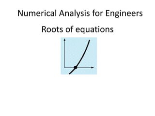
  • 1. Numerical Analysis for Engineers Roots of equations
  • 2. Roots of equations The solution of f(x) is given by the quadratic formula: The values of x’s are called roots of the function f(x) and they represent the values of x that make f(x) =0. For this reason roots are called sometimes zeros of the equation. Although the quadratic formula is handy for solving f(x), there are many other functions for which the root can’t be determined so easily. For these cases we are going to study Numerical methods that provide different means to obtain the answer.
  • 3. Roots of equations Nonlinear Equation Solvers Bracketing Graphical Open Methods Bisection False Position (Regula-Falsi) Newton Raphson Secant
  • 4. Graphical methods • Make a plot of f(x) and see when f(x) crosses the x axis. • This point represents the value of x for which f(x)=0
  • 5. Example • Use the graphical approach to determine the root of f(x)=x-14.5 x F(x) 4 -10.5 8 -6.5 12 -2.5 16 1.5 20 5.5 -12 -10 -8 -6 -4 -2 0 2 4 6 8 0 2 4 6 8 10 12 14 16 18 20 22 Eng. Muhannad Al-Jabi
  • 6. Bracketing Methods (Or, two point methods for finding roots) • Two initial guesses for the root are required. These guesses must “bracket” or be on either side of the root. • This method is based on the fact that a function typically changes it’s sign in the vicinity of a root. • If one root of a real and continuous function, f(x)=0, is bounded by values x=xl, x =xu then f(xl) . f(xu) <0. (The function changes sign on opposite sides of the root) Eng. Muhannad Al-Jabi
  • 7. Nonlinear Equation Solvers Bracketing Graphical Open Methods Bisection False Position (Regula-Falsi) Newton Raphson Secant
  • 8. 1. The Bisection Method For the arbitrary equation of one variable, f(x)=0 Step1. Choose lower xl and upper xu guesses for the root such that function changes sign over the interval. this can be checked by ensuring that f(xl).f(xu) <0. Step2. Estimate the root xr by evaluating xr = (xl+xu)/2 Step3. Determine in which subinterval the root lies: +ve -ve Xl Xr Xu
  • 9. Eng. Muhannad Al-Jabi a. If f(xl). f(xr) < 0, the root lies in the lower interval, then xu= xr and go to step 2. b. If f(xl). f(xr)> 0, root lies in the upper interval, then xl=xr go to step 2. c. If f(xl). f(xr) = 0, then root is xr and terminate. Step 4. Compare es with ea where Step 5. If ea< es, stop. Otherwise repeat the process.
  • 11. Example If the speed of a falling parachutist of mass m is given by the following equation m:the mass c: drag coefficient g: gravity acceleration t: time in seconds Eng. Muhannad Al-Jabi ) 1 ( * )* ( t m c e c g m v   
  • 12. Example Determine the drag coefficient c needed for a parachutist of mass=68.1kg to have a velocity of 40m/s after free falling for time t=10s and the gravity acceleration=9.8, by using bisection method on the interval[12,16] and εs=0.5% The equation will be Eng. Muhannad Al-Jabi 40 ) 1 ( 8 . 9 * 1 . 68 10 )* 1 . 68 (     c e c v
  • 13. Solution • We need to formulate the function Eng. Muhannad Al-Jabi 0 40 ) 1 ( 8 . 9 * 1 . 68 ) ( 10 )* 1 . 68 (      c e c c v
  • 14. Solution n xl xu xr f(xl) f(xr) f(xl).f(xr) Єa(%) 1 12 16 14 6.066936 1.568699 >0 2 14 16 15 1.568699 -0.42484 <0 6.666667 3 14 15 14.5 1.568699 0.552319 >0 3.448276 4 14.5 15 14.75 0.552319 0.058954 >0 1.694915 5 14.75 15 14.875 0.058954 -0.18413 <0 0.840336 6 14.75 14.875 14.8125 0.058954 -0.06288 <0 0.421941 If f(xl). f(xr) < 0, The root lies in the lower interval, then xu= xr If f(xl). f(xr) > 0, The root lies in the upper interval, then xl=xr If f(xl). f(xr) = 0, Then the root is xr and terminate
  • 15. Evaluation of Method Advantages • Easy • Always find root • Number of iterations required to attain an absolute error can be computed a priori. Disadvantages • Slow • Know a and b that bound root • Multiple roots • No account is taken of f(xl) and f(xu), if f(xl) is closer to zero, it is likely that root is closer to xl . Eng. Muhannad Al-Jabi
  • 16. Example Find the root of the function by using bisection method In the interval [0,10], iterate until εa falls below 0.5% 6 ) ( 2    x x x f Eng. Muhannad Al-Jabi
  • 17. Solution-a n xl xu xr f(xl) f(xu) f(xr) ea 1 0 10 5 -6 104 24 2 0 5 2.5 -6 24 2.75 100 3 0 2.5 1.25 -6 2.75 -3.1875 100 4 1.25 2.5 1.875 -3.1875 2.75 -0.60938 33.33333 5 1.875 2.5 2.1875 -0.60938 2.75 0.972656 14.28571 6 1.875 2.1875 2.03125 -0.60938 0.972656 0.157227 7.692308 7 1.875 2.03125 1.953125 -0.60938 0.157227 -0.23218 4 8 1.953125 2.03125 1.992188 -0.23218 0.157227 -0.039 1.960784 9 1.992188 2.03125 2.011719 -0.039 0.157227 0.058731 0.970874 10 1.992188 2.011719 2.001953 -0.039 0.058731 0.009769 0.487805 Eng. Muhannad Al-Jabi
  • 18. Eng. Muhannad Al-Jabi 2. The False-Position Method (Regula-Falsi) If a real root is bounded by xl and xu of f(x)=0, then we can approximate the solution by doing a linear interpolation between the points [xl, f(xl)] and [xu, f(xu)] to find the xr value The fact that the replacement of the curve by a straight line gives a “false position “ of the root is the origin of the name.
  • 19. Procedure 1. Find a pair of values of x, xl and xu such that f(xl) *f(xu)<0. 2. Using the similar triangles shown in the figure, the intersection of the straight line with the x – axis can be estimated as So estimate the value of the root from the following formula and evaluate f(xr). u r u l r l x x x f x x x f    ) ( ) ( ) ( ) ( ) )( ( u l u l u u r x f x f x x x f x x    
  • 20. Eng. Muhannad Al-Jabi 3. Use the new point to replace one of the original points, keeping the two points on opposite sides of the x axis. If f(xr)*f(xl)<0 then xu=xr If f(xr)*f(xl)>0 then xl=xr If f(xr)=0 then you have found the root and need go no further!
  • 21. 4. See if the new xl and xu are close enough for convergence to be declared. If they are not go back to step 2. • Why this method? – Faster – Always converges for a single root.
  • 22. Example Determine the real roots of by using the a) False Position Method b) Bisection Method 5 4 3 2 65 . 0 9 4 . 45 88 3 . 82 26 ) ( x x x x x x f        5 . 0  L x 0 . 1  u x 0 . 1  u x 5 . 0  L x
  • 23. Solution - False Position Method n Xl Xu Xr f(Xl) f(Xr) f(xl).f(xr) 1 0.5 1 0.62149 -1.71719 0.774501 < 0 2 0.5 0.62149 0.583727 -1.71719 0.084938 < 0 6.46934% 3 0.5 0.583727 0.579781 -1.71719 0.008812 < 0 0.68064% 4 0.5 0.579781 0.579373 -1.71719 0.000909 < 0 0.0703% a e 5 . 0  L x 0 . 1  u x ) ( ) ( ) )( ( u l u l u u r x f x f x x x f x x    
  • 24. Solution - Bisection Method 5 . 0  L x 0 . 1  u x n xl xu xr f(xl) f(xr) f(xl).f(xr) Єa 1 0.5 1 0.75 -1.71719 2.684717 < 0 2 0.5 0.75 0.625 -1.71719 0.835182 < 0 20% 3 0.5 0.625 0.5625 -1.71719 -0.33419 > 0 11.1111% 4 0.5625 0.625 0.59375 -0.33419 0.27473 < 0 5.2631% xr = (xl+xu)/2 At n= 4 the Єa equals 0.07% in case of using False position while it equals 5.2% in case of using Bisection Method => The False position is Faster
  • 25. Example You are designing a spherical tank to hold water for a small village. The volume of the liquid can hold can be computed as R: is the radius h:is the height if the liquid Eng. Muhannad Al-Jabi 3 3 2 2 h R h v   
  • 26. Example If R=3m, determine the depth the tank must be filled so that it holds 30m3 a) By using bisection method, five iterations b) By using false position method , five iterations Eng. Muhannad Al-Jabi 0 30 3 3 * 3 2 ) ( 2     h h h f 
  • 27. Solution- By using bisection method xl xu xr f(xl) f(xu) f(xr) ea 0 6 3 -30 196.08 83.04 0 3 1.5 -30 83.04 5.325 100 0 1.5 0.75 -30 5.325 -20.2856 100 0.75 1.5 1.125 -20.2856 5.325 -9.13617 33.33333 1.125 1.5 1.3125 -9.13617 5.325 -2.27815 14.28571 Eng. Muhannad Al-Jabi
  • 28. Solution- By using false position method xl xu xr f(xl) f(xu) f(xr) ea 0 6 0.796178 -30 196.08 -19.1138 0.796178 6 1.258389 -19.1138 196.08 -4.33745 36.73036 1.258389 6 1.361008 -4.33745 196.08 -0.37928 7.539885 1.361008 6 1.369964 -0.37928 196.08 -0.02335 0.653735 1.369964 6 1.370515 -0.02335 196.08 -0.00139 0.04023 Eng. Muhannad Al-Jabi
  • 29. Example Determine the value of By using 5 iterations of a)false position method b) Bisection method The estimated root will be between 4 and 5 why? Eng. Muhannad Al-Jabi 18 0 18 ) (    x x f
  • 30. Solution -False position method xl xu xr f(xl) f(xr) f(xl)*f(xr) ea 4 5 4.242641 -0.24264 0 0 Eng. Muhannad Al-Jabi ) ( ) ( ) )( ( u l u l u u r x f x f x x x f x x     0 18 ) (    x x f
  • 31. Solution - Bisection method xl xu xr f(xl) f(xr) f(xl)*f(xr) ea 4 5 4.5 -0.24264 0.257359 < 0 4 4.5 4.25 -0.24264 0.007359 < 0 5.882353 4 4.25 4.125 -0.24264 -0.11764 > 0 3.030303 4.125 4.25 4.1875 -0.11764 -0.05514 > 0 1.492537 4.1875 4.25 4.21875 -0.05514 -0.02389 > 0 0.740741 Eng. Muhannad Al-Jabi
  • 32. Nonlinear Equation Solvers Bracketing Graphical Open Methods Bisection False Position (Regula-Falsi) Newton Raphson Secant
  • 33. Open Methods • Open methods start with a starting point or the initial guess. • Because the open methods do not bracketing the root, they may be converges or diverges. • On the other hand open methods are faster in finding the root. ( more efficient). Eng. Muhannad Al-Jabi
  • 34. Bracketing methods Always Converges as the root is Constrained within the interval Prescribed by xl and xu. The open method depicted in figure b And c . The method can be either diverge or converge diverge converge
  • 36. Newton-Raphson Method • Or it can be derived based on Taylor series expansion: ) ( ) ( ) ( 0 g, Rearrangin 0 ) f(x when x of value the is root The ) )( ( ) ( ) ( 1 1 1 i 1 i 1 1 i i i i i i i i i i i i i x f x f x x x x ) (x f ) f(x Rn x x x f x f x f                   
  • 37. Example • Find the root of f(x) using the Newton Raphson method Solution: x e x f x    ) ( 0 0  x 1 ) ( '    x e x f 1 1         i i x i x i i e x e x x % 1 . 0  s e i Xi εa 0 0 1 0.5 100 2 0.566311 11.70929 3 0.567143 0.146729 4 0.567143 2.21E-05 ) ( ) ( 1 i i i i x f x f x x    
  • 38. Use the simple fixed point iteration method to find the root using fixed point iteration Solution: Eng. Muhannad Al-Jabi x e x f x    ) ( 0 0  x i Xi εa 0 0 1 1,00 100 2 0.367879 171 3 0.692201 46 4 0.500471 38 5 0.606244 17 6 0.5453 11 7 0.579612 5.9 8 0.560115 3.4 9 0.571143 1.93 10 0.564870 1.11 ) ( 1 i i x g x   Thus, the approach rapidly converges on the true root. Notice that the Єa at each iteration Decreases much faster than it does in simple fixed point iteration.
  • 39. Eng. Muhannad Al-Jabi • A convenient method for functions whose derivatives can be evaluated analytically. It may not be convenient for functions whose derivatives cannot be evaluated analytically.
  • 40. • The need to evaluate of f(x) and it’s derivative (slope) . • Simple and faster than other methods. • Convergence depends on the initial guess (not guaranteed). • Multiple root. • Poor predication makes the convergence very slow!!! • Newton Raphson method is quadratically convergent. That is the error is roughly proportional to the square of the previous error as shown. i t r r i t E x f x f E , 2 ' ' 1 , ) ( ' 2 ) (    Newton Raphson Method features
  • 41. Cases where The Newton-Raphson Method exhibits poor convergence
  • 42. Example • Find the root of Using Newton Raphson method. Use Try and Solution 5 . 2 7 . 1 9 . 0 ) ( 2     x x x f 5 0  x 7 . 1 8 . 1 5 . 2 7 . 1 9 . 0 2 1         i i i i i x x x x x % 1 . 0  s e 1 0  x Xi εa 1 34 97.05882 17.52773 -93.9783 9.346734 -87.5279 5.363967 -74.2504 3.569381 -50.2772 2.95593 -20.7532 2.862387 -3.26802 Xi εa 5 3.424658 -46 2.924357 -17.1081 2.861147 -2.20925 2.860105 -0.03644 We can see that for this function, newton raphson method is faster when starting with X0 =5 7 . 1 8 . 1 ) ( '    x x f
  • 43. Example • Use Newton-Raphson method to find the root of F(x)=-x2+1.8x+25 Starting with x0=5 and use εs=5%.
  • 44. Solution- Newton-Raphson method x f(x) f'(x) ea 5 -13.5 -8.2 3.353659 -2.71044 -4.90732 49.09091 2.801332 -0.30506 -3.80266 19.71656 2.721108 -0.00644 -3.64222 2.948204 8 . 1 2 5 . 2 8 . 1 2 1        i i i i i x x x x x Starting with x0=5 and use εs=5%. 8 . 1 2 ) ( ' 5 . 2 8 . 1 ) ( 2        x x f x x x f
  • 45. Additional features are necessary for improving Newton Raphson method algorithm
  • 46. The Secant Method • As introduced in the Newton Raphson method, There is a need to calculate the first derivative of f(x) which is not convenient in some cases. • For these cases the derivative can be approximated as: This approximation can be substituted in the Newton Raphson equation to yield the following iterative equation: 1 1 1 ) ( ) ( ) (        i i i i i i i x x x f x f x f x x 1 1) ( ) ( ) (       i i i i i x x x f x f x f ) ( ) ( 1 i i i i x f x f x x     Newton Raphson method ) ( ) ( ) ( 1 1 1        i i i i i i i x f x f x x x f x x Slope of the secant
  • 47. The Secant Method • Requires two initial estimates of x , e.g, xo, x-1. However, because f(x) is not required to change signs between estimates, it is not classified as a “bracketing” method. • The secant method has the same properties as Newton’s method. Convergence is not guaranteed for all xo, f(x).
  • 48. The secant method technique is similar to the Newton-Raphson in sense that an estimate of the root is predicted by extrapolating a tangent of the function to the x-axis. The secant method uses a difference rather than a derivative to estimate the slope in each step. The slope of the secant line is the average change of f(x) over an interval [xi-1,xi] The slope of the tangent line is rate of change of f(x) at xi. Secant method Newton method
  • 50. • The Van der Waals equation of state is given as shown below: • If a = 1.33 (liter/mol)2, b = 0.0366 liter/mol, R = 0.08206 (liter.atm/mol.K) and the air is at temperature T = 223 K and pressure P = 50 atm. • Use secant method to estimate specific volume V using only three iterations? Estimate εa for each iteration? The initial guesses are V-1 = 0.1 and V0 = 0.2 .
  • 51. Vi-1 Vi Vi+1 F(Vi-1) f(Vi) f(Vi+1) ea% 0.1 0.2 0.434717 - 6.69718 - 4.69633 4.408336 46.30301 0.2 0.434717 0.321071 - 4.69633 4.408336 - 0.40567 1.601455 0.434717 0.321071 0.330647 4.408336 - 0.40567 - 0.01985 0.009803
  • 52. Example • Suppose that you have the following electrical circuit L = 5H, C=10-4 F. Find the value of R that makes the value of the capacitor charge (q) equals to 0.01 of the initial capacitor charge (q0) after 0.05 seconds from turning the switch. Use secant method with xi=250, xi-1=260, εs=0.01
  • 55. Solution xi-1 xi xi+1 ea 250 260 319.1185 18.52555 260 319.1185 327.0756 2.432807 319.1185 327.0756 328.134 0.322543 327.0756 328.134 328.1514 0.005315 Eng. Muhannad Al-Jabi ) ( ) ( ) ( 1 1 1        i i i i i i i x f x f x x x f x x
  • 56. The Difference Between The Secant method and False Position Method ) ( ) ( ) ( 1 1 1        i i i i i i i x f x f x x x f x x False Position Secant Method ) ( ) ( ) )( ( u l u l u u r x f x f x x x f x x    
  • 57. The two estimates of xl and xu Always bracket the root And the convergence is guaranteed The values are replaced in strict sequence , Xi+1 ---------> Xi Xi ---------> Xi-1 The two values can some times lie on the same side of the root which can Lead to divergence A critical difference between the methods is how one of the initial values is replaced by the new estimates !!!!!!!!!
  • 58. The figure below shows the true percent error єt for the methods to determine the roots of f(x)= exp(-x) – x .
  • 59. Multiple roots A multiple root (double, triple, etc.) occurs where the function is tangent to the x axis. For example a double result from f(x)= (x-3)(x-1)(x-1) = x³ -5x²+7x-3 This equation has a multiple root because one value of root makes the two terms equal to zero. Graphically this corresponds to the curve touching the x axis tangentially at the double root. Note: that the function touches the x axis but does not cross it at the root.
  • 60. • A multiple root (double, triple, etc.) occurs where the function is tangent to the x axis single root double roots
  • 61. Note: that the function touches the x axis but cross it at the root. In general odd multiple root crosses the axis whereas even do not.
  • 62. Problems with multiple roots • The function does not change sign at even multiple roots (i.e., m = 2, 4, 6, …) which means that Bracketing methods can’t be applied. • f (x) goes to zero - This means that Newton Raphson method and Secant method can’t be applied. A need to put a zero check for f(x) in program. • Slower convergence (linear instead of quadratic) of Newton-Raphson and secant methods for multiple roots. Modification have been applied to alleviate this problem (i.e. multiplicity of the root, m = 2, 4, 6, …) ) ( ) ( 1 i i i i x f x f m x x    
  • 63. • A more general modification is to define a new function u(x), that is equal to the ratio of the function to its first derivative as in It can be shown that this function has roots at all the same locations as the original functions. Therefore the Newton Raphson equation Can be developed to following equation for multiple roots ) ( ) ( 1 i i i i x f x f x x     ) ( ' ) ( 1 i i i i x u x u x x    ) ( ' ) ( ) ( i i x f x f x u 
  • 64. Eng. Muhannad Al-Jabi • The above equation can be written in terms of f(x) ) ( ' ' ) ( )] ( ' [ ) ( ' ) ( 2 1 i i i i i i i x f x f x f x f x f x x    
  • 65. Example • Use both standard and modified Newton Raphson methods to find the roots of a) Start at xo = 0 b) Start at xo = 4 Do five iterations only and compare the behavior of εa between standard and modified methods in part a and part b ) 1 )( 1 )( 3 ( ) (     x x x x f
  • 66. Solution part a : xo = 0 Xi εa 0 0.428571 100 0.685714 37.5 0.832865 17.66805 0.91333 8.810014 0.955783 4.441739 Standard Xi εa 0 1.105263 100 1.003082 -10.1868 1.000002 -0.30793 1 -0.00024 1 -1.4E-10 Modified We can see that the modified method is faster because there are multiple roots at x=1 and it becomes quadratically convergent. ) ( ' ' ) ( )] ( ' [ ) ( ' ) ( 2 1 i i i i i i i x f x f x f x f x f x x     ) ( ) ( 1 i i i i x f x f x x    
  • 67. Solution part b: xo = 4 Xi εa 4 3.4 -17.6471 3.1 -9.67742 3.008696 -3.03468 3.000075 -0.28736 3 -0.00249 standard Xi εa 4 2.636364 -51.7241 2.820225 6.519377 2.961728 4.777734 2.998479 1.225638 2.999998 0.050632 modified We can see that the standard method is faster because there is single root at x=3
  • 68. Systems of nonlinear equations To this point we focused on the determination of the root of a single equation. A related problem is to locate the roots of a set of simultaneous equations. f1(x1, x2, x3,…. xn)=0 f2(x1, x2, x3,…. xn)=0 fn(x1, x2, x3,…. xn)=0 Example of simultaneous non linear equations with two unknowns: x² + xy = 10 y+3xy²= 57 They can be expressed in this form u(x,y) = x² + xy – 10 =0 v(x,y)= y+3xy² - 57= 0
  • 69. Systems of nonlinear equations The solutions would be the values of x and y that make u(x,y)=0 and v(x,y)=0. Most approaches for determining such solutions are extensions of the open method for solving single equations.
  • 70. Systems of nonlinear equations Fixed point iterations Let us we have two equations u(x,y)=0 and v(x,y)=0. From u(x,y) we can extract x to be Xi+1 = gu(xi,yi) And from v(x,y) we can extract y to be Yi+1=gv(xi+1,yi) Eng. Muhannad Al-Jabi
  • 71. Systems of nonlinear equations The convergence depends on the manner in which the equations are formulated and the initial guesses Convergence of fixed point iterations This fixed point iteration has limited utility for solving non-linear systems. However, this method is useful for solving linear systems.
  • 72. Example Solve the following system of nonlinear equations using fixed point iterations, for two iterations only and start with x=1.5,y=3.5 0 57 3 ) , ( 0 10 ) , ( 2 2         xy y y x v xy x y x u We can see that x and y can be extracted by multiple ways
  • 73. Solution-diverges x y Єax Єay 1.5 3.5 2.214286 -24.375 32.25806 -114.359 -0.20911 429.7136 -1158.93 105.6724 0.02317 -12778 1002.5 -103.363 gu (x,y) gv(x,y) y x x 2 10   2 3 57 xy y   Diverges
  • 74. Solution-converges x y εax εay 1.5 3.5 2.179449 2.860506 31.17528 22.35598 1.940534 3.049551 12.31185 6.1991 2.020456 2.983405 3.955661 2.217129 gu (x,y) gv(x,y) xy x   10 x y y 3 57   converges
  • 76. Example Find the intersection point of the line • y=x And the circle • x2+y2=5 By using Newton-Raphson method with 4 iterations only. x0=1,y0=0.5
  • 77. Solution We need to formulate the problem on the form u(x,y)= x2+y2-5=0 v(x,y)=y-x=0 And in each iteration we need to calculate
  • 78. Solution x v y u y v x u y u v y v u x x i i i i i i i i i i                 1 x v y u y v x u x v u x u v y y i i i i i i i i i i                 1 u(x0, y0)=u(1,0.5)= 12+0.52-5= - 3.75 v(x0, y0)=v(1,0.5)=0.5-1= - 0.5 ∂u0 / ∂x =2x0 =2(1)=2 x0=1, y0=0.5 ∂u0 / ∂y =2y0=2(0.5)=1 ∂v0 / ∂x =-1 ∂v0 / ∂y =1 3            x v y u y v x u Jacobian i i i i 2.083333 3 ) 1 )( 5 . 0 ( ) 1 ( 75 . 3 1 1       x 4166667 . 0 3 1 ) 75 . 3 ( 2 ) 5 . 0 ( 5 . 0 1        y
  • 79. Solution x v y u y v x u y u v y v u x x i i i i i i i i i i                 1 x v y u y v x u x v u x u v y y i i i i i i i i i i                 1 i xi yi u(xi, yi) v(xi, yi) ∂ui / ∂x ∂ui / ∂y ∂vi/ ∂x ∂vi / ∂y jacobian 0 1 0.5 -3.75 -0.5 2 1 -1 1 3 1 2.083333 2.083333 3.680556 0 4.166667 4.166667 -1 1 8.333333 2 1.641667 1.641667 0.390139 0 3.283333 3.283333 -1 1 6.566667 3 1.582255 1.582255 0.00706 0 3.164509 3.164509 -1 1 6.329019 4 1.581139 1.581139 2.49E-06 0 3.162278 3.162278 -1 1 6.324557
  • 80. Example Use Newton-Raphson method to solve the following equations, starting with x=1,y=1, for two iterations only Eng. Muhannad Al-Jabi 0 cos 2 ) , ( 0 1 ) , ( 2        y x y x v y x y x u x x u 2    1     y u x x v sin 2     1     y v
  • 81. solution x y 1 1 0.750364 1.500728 0.715397 1.51057 0.714621 1.510683 0.714621 1.510683 Eng. Muhannad Al-Jabi
  • 82. f(r)= 40r + -1 =0 Example : Use the Newton Raphson Method to find the monthly interest rate (r) correct to 4 significant figures. Use initial guess at r0=0.015. ri f(ri) f’(ri) r i+1 0.015 9.2959*10-3 15.805 0.01441184 0.01441 2.2707*10-4 14.9316 0.01439499 0.01439 -7.126*10-5 14.90144 0.01439478 We stopped here as 4 similar significant figures has been obtained.
  • 83. Example Find the intersection point of the line • y=x And the circle • x2+y2=5 By using fixed point iteration method with 4 iterations only Eng. Muhannad Al-Jabi
  • 85. Solution i xi xi+1 yi yi+1 0 1 2.179449 0.5 2.179449 1 2.179449 0.500000 2.179449 0.500000 2 0.500000 2.179449 0.500000 2.179449 3 2.179449 0.500000 2.179449 0.500000 4 0.5 0.5 Eng. Muhannad Al-Jabi 5 . 0 1 0 0   y x ) , ( ) , ( ) , ( 5 ) , ( 1 1 1 2 i i v i v i i u i u y x g y x y x g y x g x y y x g          
  • 86. Question 6.1 Use simple fixed point iteration to locate the root of Use the initial guess of x0=0.5 and εs=0.01 Eng. Muhannad Al-Jabi x x x f   ) sin( 2 ) (
  • 87. Solution x g(x) ea 0.5 1.299274 1.299274 1.817148 61.51697 1.817148 1.950574 28.49926 1.950574 1.969743 6.840367 1.969743 1.972069 0.973152 1.972069 1.972344 0.117966 1.972344 1.972377 0.013958 1.972377 1.97238 0.001647 Eng. Muhannad Al-Jabi ) sin( 2 ) ( x x g  ) ( 1 i i x g x  
  • 88. Question 6.2 Determine the root of a)Graphically b)Fixed point iteration method (three iterations, x0=3). c)Newton-Raphson method(three iterations x0=3). d) Secant method(three iterations, xi-1=3,xi=4) e)Modified secant method( three iterations ,x0=3,δx=0.01) Eng. Muhannad Al-Jabi 5 7 . 17 7 . 11 2 ) ( 2 3     x x x x f
  • 89. Solution b : Fixed point iteration method Eng. Muhannad Al-Jabi 2 2 2 5 7 . 17 7 . 11 ) ( x x x x g    x g(x) ea 3 3.177778 3.177778 3.312602 5.594406 3.312602 3.406209 4.070042 3.406209 3.467279 2.748134
  • 90. Solution c: Newton-Raphson method x f(x) fp(x) ea 3 -3.2 1.5 5.133333 48.09007 55.68667 41.55844 4.26975 12.95624 27.17244 20.22562 3.792934 2.947603 15.26344 12.57115 Eng. Muhannad Al-Jabi
  • 91. Solution d : Secant method(three iterations, xi-1=3,xi=4) xi-1 xi xi+1 ea 3 4 3.326531 20.2454 4 3.326531 3.481273 4.444986 3.326531 3.481273 3.586275 2.927903 Eng. Muhannad Al-Jabi
  • 92. Solution e : Modified secant method x ea 3 5.047083 40.55972 4.221812 19.5478 3.77217 11.91997 Eng. Muhannad Al-Jabi
  • 93. Question 6.8 Determine the root of x3.5=80 using secant method with xi-1=3,xi=4 and εs=0.1 Eng. Muhannad Al-Jabi
  • 94. Solution xi-1 xi xi+1 ea 3 4 3.409119 17.33237 4 3.409119 3.482859 2.117227 3.409119 3.482859 3.497825 0.427858 3.482859 3.497825 3.497355 0.013436 Eng. Muhannad Al-Jabi F(x)=x3.5-80=0
  • 95. Question 6.12 Determine the roots of the following simultaneous nonlinear equations using a) Fixed point iteration b) Newton-Raphson method Eng. Muhannad Al-Jabi x xy y x x y       5 75 . 0 2
  • 96. Solution-Fixed point iteration Eng. Muhannad Al-Jabi x x y y x g y x y x g x xy y y x v x x y y x u x xy y x x y v u 5 ) , ( 75 . 0 ) , ( 5 ) , ( 75 . 0 ) , ( 5 75 . 0 2 2                   
  • 97. Solution-Fixed point iteration x y eax eay 1.2 1.2 0.866025 -0.07713 38.56406 -1655.85 1.301212 0.211855 33.44473 136.4061 1.356229 0.168758 4.056602 25.53745 1.391931 0.175752 2.564889 3.979279 1.402205 0.174932 0.732725 0.468668 1.406155 0.175119 0.280937 0.106804 1.407493 0.175116 0.09503 0.001675 Eng. Muhannad Al-Jabi
  • 98. Solution-Newton-Raphson method Eng. Muhannad Al-Jabi x dy dv y dx dv dy du x dx du x xy y y x v x x y y x u 5 1 1 5 1 1 2 5 ) , ( 75 . 0 ) , ( 2              
  • 99. Solution :Newton-Raphson method Eng. Muhannad Al-Jabi x y u v dux duy dvx dvy jacobian eax eay 1.2 1.2 0.69 7.2 1.4 1 5 7 4.8 1.69375 -0.18125 0.243789 -3.40996 2.3875 1 -1.90625 9.46875 24.51289 29.15129 -762.069 1.460471 0.131914 0.054419 -0.36527 1.920942 1 -0.34043 8.302356 16.28878 15.97285 237.4 1.410309 0.173854 0.002516 -0.01052 1.820618 1 -0.13073 8.051545 14.78952 3.556815 24.12343 1.408228 0.175126 4.33E-06 -1.3E-05 1.816456 1 -0.12437 8.04114 14.73075 0.147781 0.726703 1.408225 0.175128 1.06E-11 -2.6E-11 1.816449 1 -0.12436 8.041124 14.73066 0.000232 0.000912 1.408225 0.175128 0 0 1.816449 1 -0.12436 8.041124 14.73066 5.38E-10 1.78E-09
  • 100. Question 6.13 Determine the roots of the simultaneous nonlinear equations Use graphical approach to obtain your initial guesses. Then use Newoton-Raphson method to refine your estimate Eng. Muhannad Al-Jabi 16 5 ) 4 ( ) 4 ( 2 2 2 2       y x y x
  • 102. Solution x y u v dux duy dvx dvy jacobian eax eay 3 2.5 -1.75 -0.75 -2 -3 6 5 8 4.375 1 4.140625 4.140625 0.75 -6 8.75 2 54 31.42857 150 3.761574 1.613426 0.752583 0.752583 -0.47685 -4.77315 7.523148 3.226852 34.37037 16.30769 38.02009 3.586404 1.788596 0.061369 0.061369 -0.82719 -4.42281 7.172808 3.577192 28.76493 4.884283 9.793722 3.569336 1.805664 0.000583 0.000583 -0.86133 -4.38867 7.138672 3.611328 28.21876 0.478178 0.945235 3.569171 1.805829 5.46E-08 5.46E-08 -0.86166 -4.38834 7.138342 3.611658 28.21347 0.004628 0.009147 3.569171 1.805829 0 0 -0.86166 -4.38834 7.138342 3.611658 28.21347 4.33E-07 8.57E-07 Eng. Muhannad Al-Jabi
  • 103. Question 6.14 Repeat the previous question for Eng. Muhannad Al-Jabi x y x y cos 2 1 2   
  • 104. Solution Eng. Muhannad Al-Jabi 1 sin 2 1 2 cos 2 ) , ( 1 ) , ( 2           dy dv x dx dv dy du x dx du x y y x v x y y x u
  • 105. Solution x y u v dux duy dvx dvy jacobian eax eay 0.5 1 -0.25 -0.75517 -1 1 0.958851 1 -1.95885 0.757888 1.507888 -0.06651 0.05531 -1.51578 1 1.374779 1 -2.89056 34.02723 33.6821 0.715745 1.510515 -0.00178 0.001307 -1.43149 1 1.31236 1 -2.74385 5.887993 0.173915 0.714622 1.510683 -1.3E-06 9.53E-07 -1.42924 1 1.310664 1 -2.73991 0.157226 0.011098 0.714621 1.510683 -6.5E-13 4.94E-13 -1.42924 1 1.310662 1 -2.7399 0.000113 7.07E-06 0.714621 1.510683 -1.1E-16 2.22E-16 -1.42924 1 1.310662 1 -2.7399 5.86E-11 3.65E-12 0.714621 1.510683 0 0 -1.42924 1 1.310662 1 -2.7399 1.55E-14 0
  • 106.
  • 107. Civil Engineering application Question 8.18 Suppose that you have a uniform beam subject to linearly increasing distributed load. The equation for the resulting elastic curve Use the bisection method to determine the point of maximum deflection( that is, the value of x where dy/dx=0). Then substitute this value of x in the equation to get the maximum deflection. L=600cm, E=50000kN/cm2,I=30000cm4, ω0=2.5kN/cm. use εs=10% ) 2 ( 120 4 3 2 5 0 x L x L x EIL y     
  • 109. Solution Eng. Muhannad Al-Jabi ) 2 ( 120 4 3 2 5 0 x L x L x EIL y      0 600 * 600 * 6 5 ) ( 0 3 * 2 5 0 ) 3 * 2 5 ( 120 4 2 2 4 4 2 2 4 4 2 2 4 0               x x x f L x L x L x L x EIL dx dy 
  • 110. Graphical solution x f(x) 0 -360000 1 1799995 2 8279920 3 19079595 4 34198720 It seems that the maximum deflection occurs within the first centimeter
  • 111. Solution bisection method xl xu xr f(xl) f(xr) ea 0 1 0.5 -360000 179999.7 0 0.5 0.25 -360000 -225000 100 0.25 0.5 0.375 -225000 -56250.1 33.33333 0.375 0.5 0.4375 -56250.1 53437.32 14.28571 0.375 0.4375 0.40625 -56250.1 -3515.76 7.692308 The maximum deflection =-4.875*10-07 εs=10%
  • 112. Environmental Engineering application Question 8.19 The following equation can be used to compute the oxygen level c (mg/L) in a river downstream from a sewage discharge Where x is the distance in kilometers. ) ( 20 10 5 . 0 15 . 0 x x e e c     
  • 113. a) Determine the distance downstream where the oxygen level first falls to a reading of 5mg/L. Hint: it will be within the first 2 kilometers of the discharge. Determine your answer to 10% error b) Determine the distance at which the concentration is minimum, and what is the concentration at that location. Determine your answer to 5% error Question 8.19
  • 114. Solution -a Since the answer will be within the first 2 kilometers, we can use bracketing method such as the bisection method with x0=0 and xu =2. 0 5 ) ( 20 10 ) ( 5 . 0 15 . 0        x x e e x f
  • 115. Solution -a xl xu xr f(xl) f(xu) f(xr) ea 0 2 1 5 -2.45878 -0.08355 0 1 0.5 5 -0.08355 2.021146 100 0.5 1 0.75 2.021146 -0.08355 0.873839 33.33333 0.75 1 0.875 0.873839 -0.08355 0.373001 14.28571 0.875 1 0.9375 0.373001 -0.08355 0.139379 6.666667
  • 116. Solution -b x f’(x) 0 0.35 1 0.174159 2 0.072817 3 0.015921 4 -0.01465 0 ) 5 . 0 15 . 0 ( 20 ) ( ' 5 . 0 15 . 0        x x e e x f 0 ) 5 . 0 15 . 0 ( ) ( ' 5 . 0 15 . 0       x x e e x f
  • 117. Solution -b xl xu xr f(xl) f(xu) f(xr) ea 3 4 3.5 0.015921 -0.01465 -0.00185 3 3.5 3.25 0.015921 -0.00185 0.006332 7.692308 3.25 3.5 3.375 0.006332 -0.00185 0.002078 3.703704 The minimum concentration occurs at x=3.375 and it equals to 1.644595 We select xl =3 and xu =4 as the curve changes it’s sign around it
  • 118. A total charge Q is uniformly distributed around a ring shaped conductor with radius a. A charge q is located at a distance x from the center of the ring. The force exerted on the charge by the ring is given by Where e0 =8.85*10-12 C2/(Nm2). Find the distance x where the force is 1.25N if Q and q are 2*10-5C for a ring with a radius of 0.9m 2 / 3 2 2 0 ) ( 4 1 a x qQx e F    Electrical Engineering application Question 8.31
  • 119. Question 8.31 Use bisection method with εs=10% 0 25 . 1 ) ( 4 1 ) ( 2 / 3 2 2 0     a x qQx e x f 
  • 120. Solution xl xu xr f(xl) f(xu) f(xr) ea 0 1 0.5 -1.25 0.227778 0.398687 0 0.5 0.25 -1.25 0.398687 -0.14613 100 0.25 0.5 0.375 -0.14613 0.398687 0.205943 33.33333 0.25 0.375 0.3125 -0.14613 0.205943 0.050454 20 0.25 0.3125 0.28125 -0.14613 0.050454 -0.04276 11.11111 0.28125 0.3125 0.296875 -0.04276 0.050454 0.005129 5.263158

Editor's Notes

  1. 11-12.5 17 sep.
  2. 10 -11 11sep.
  3. The fact that the replacement of the curve by a straight line gives a “false position “ of the root is the origin of the name.
  4. 8-9.5 12 sep.
  5. 10-11 16sep.
  6. 8-9.5 19sep
  7. To avoid the need of calculating the first derivative of f(x) at each step, we exploit the relationship between secant line and tangent line . The slope of the secant line is the average change of f(x) over an interval [a,b]. The slope of the tangent line is rate of change of f(x) at b.
  8. u(x) contains only single roots even though f(x) may have multiple roots
  9. 10-11 1-2 25sep
  10. 11-12.5 26sep
  11. 8.-9.5 26sep, I skipped the fixed point iteration
  12. 1-2 26sep
  13. Surface tension
  14. The permittivity of free space