Download as PDF, PPTX

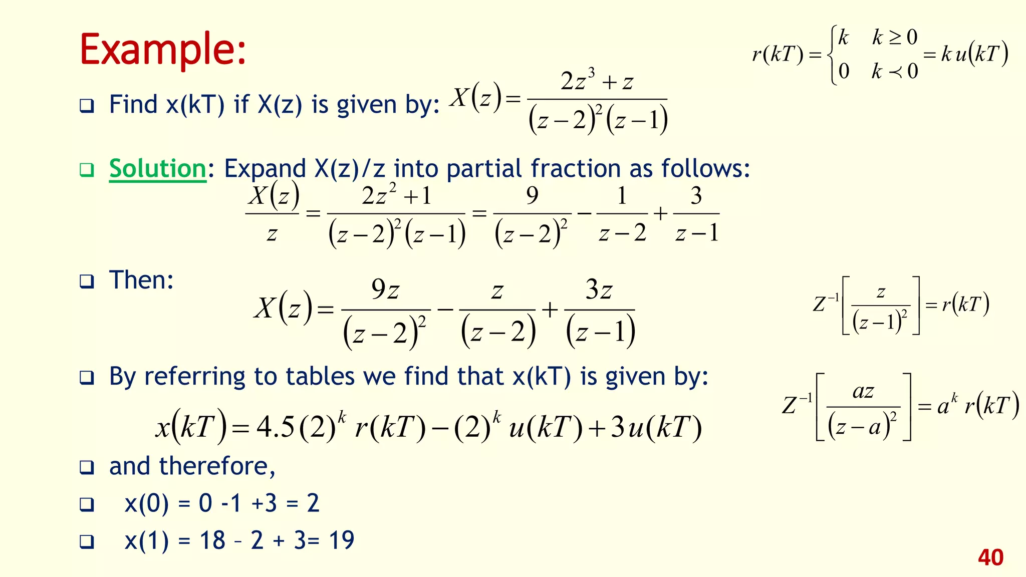
![z-transform of kaku[k]
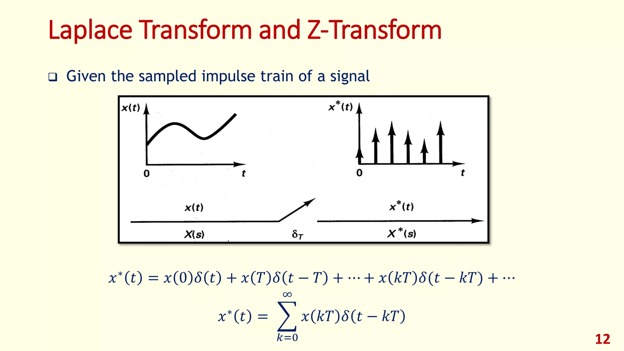
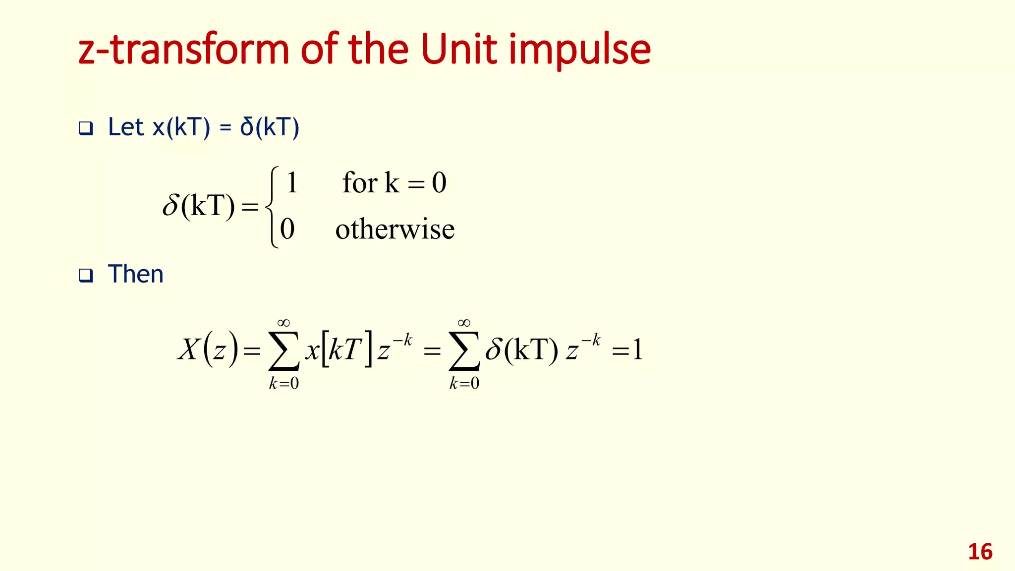
Let x(kT) = k ak u(kT)
Then
20
0kfor0
0kfor
(kT)
k
k ka
uka
000
k(kT))(
k
kk
k
kk
k
k
zazukazkTxzX
221
0
1
)()1(
1
)(k
az
z
az
azzX
k
k
](https://image.slidesharecdn.com/dcs-lec02-z-transform-191118221227/75/Dcs-lec02-z-transform-20-2048.jpg)
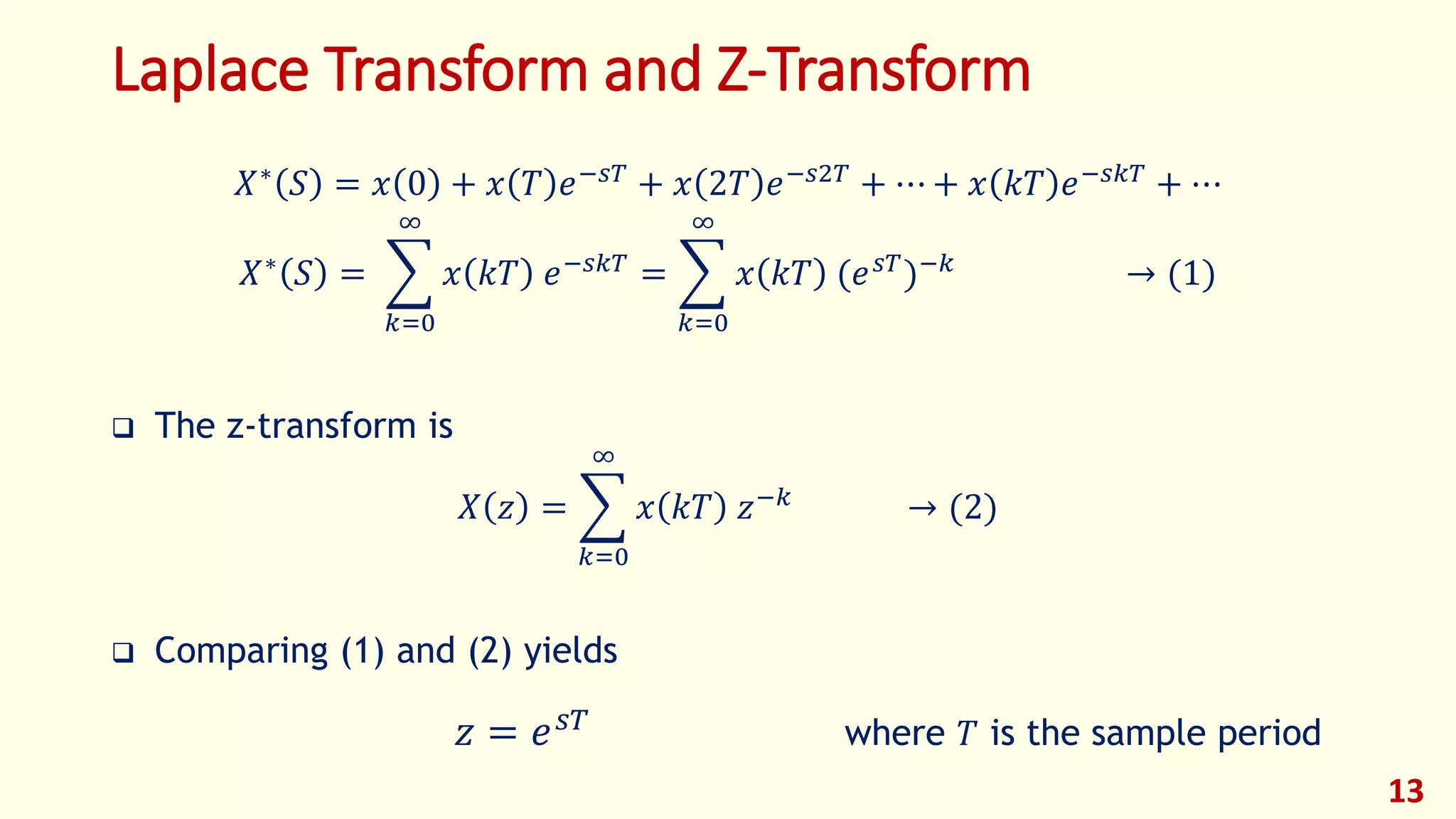
![Z-Transform Properties: Time Left Shifting (Time Advance)
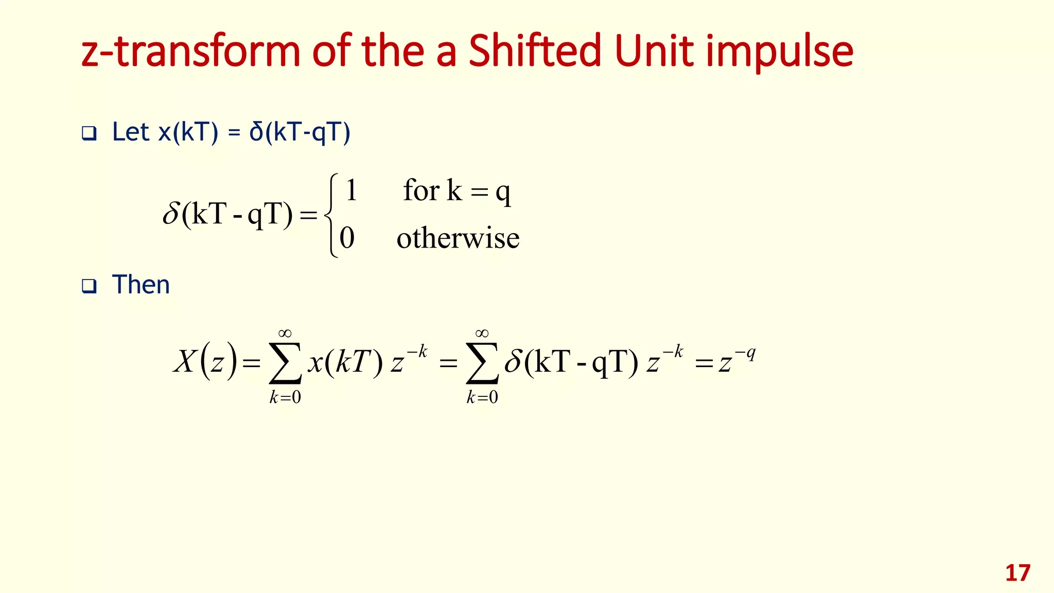
Example:
26
])([)(
1
0
n
k
knZ
zkTxzXznTkTx
))2(()2.0()( )2(
TkukTx Tk
])(
2.01
1
[)(
1
0
1
2
k
k
zkTx
z
zZX
1
1
1
2
2.01
04.0
)]2.01(
2.01
1
[)(
z
z
z
zZX](https://image.slidesharecdn.com/dcs-lec02-z-transform-191118221227/75/Dcs-lec02-z-transform-26-2048.jpg)
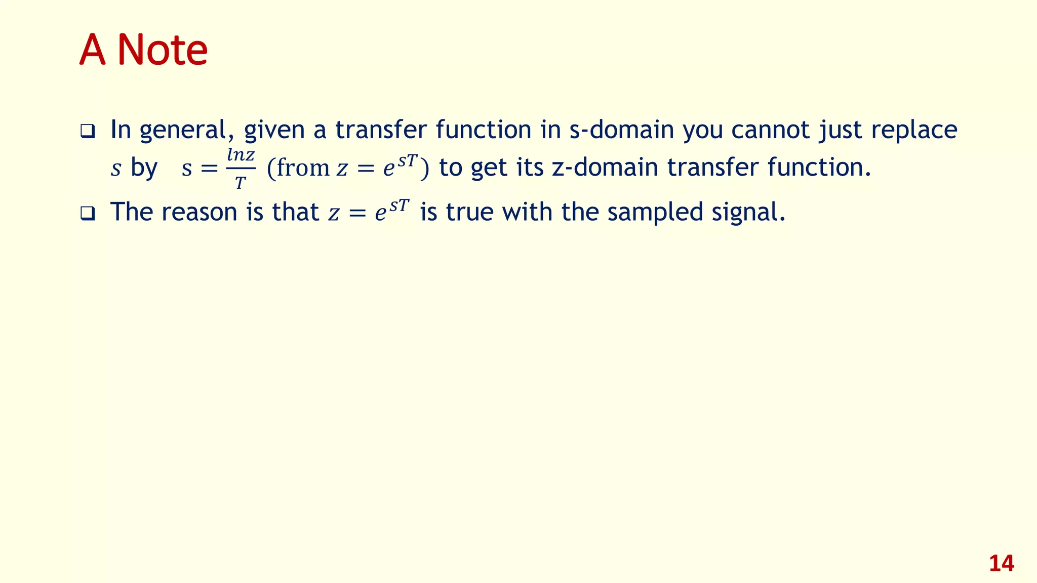
![Z-Transform Properties: Initial and Final Value Theorems
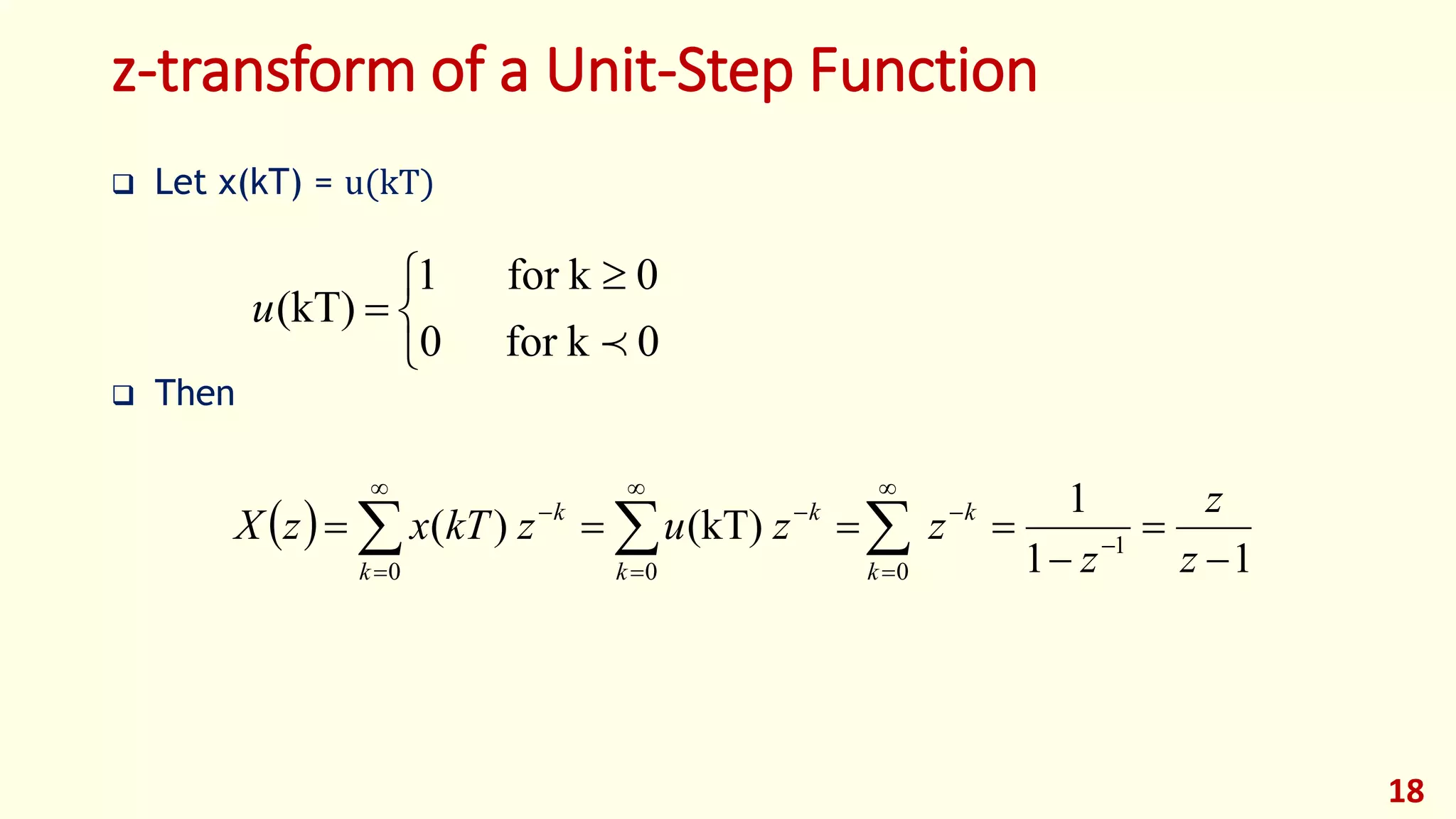
Initial Value Theorem:
The value of x(n) as k → 0 is given by:
Final Value Theorem:
The value of x(n) as k → is given by:
30
)(limlim)0(
0
zXkTxx
zk
)]()1[(limlim)(
1
zXzkTxx
zk
](https://image.slidesharecdn.com/dcs-lec02-z-transform-191118221227/75/Dcs-lec02-z-transform-30-2048.jpg)

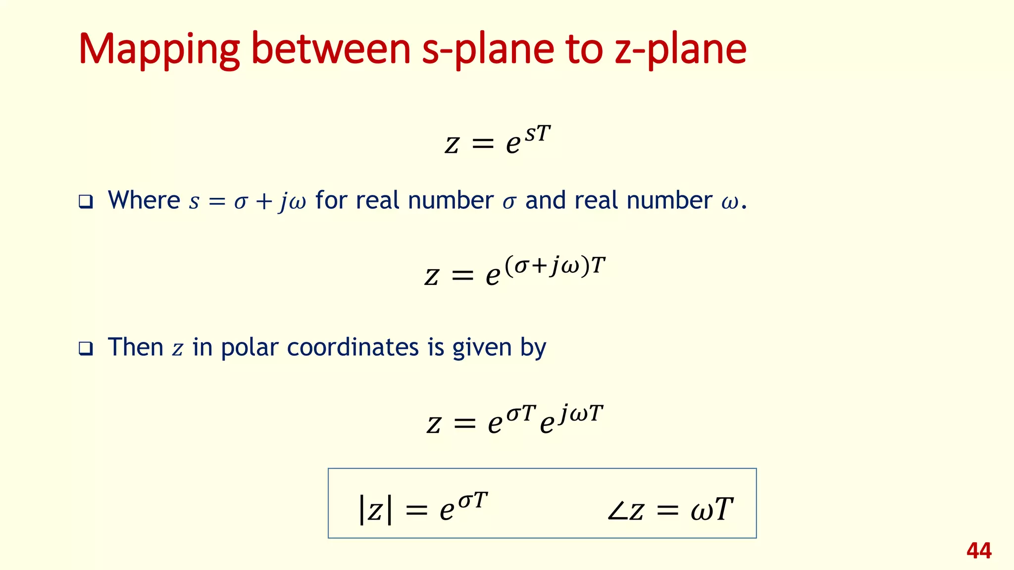
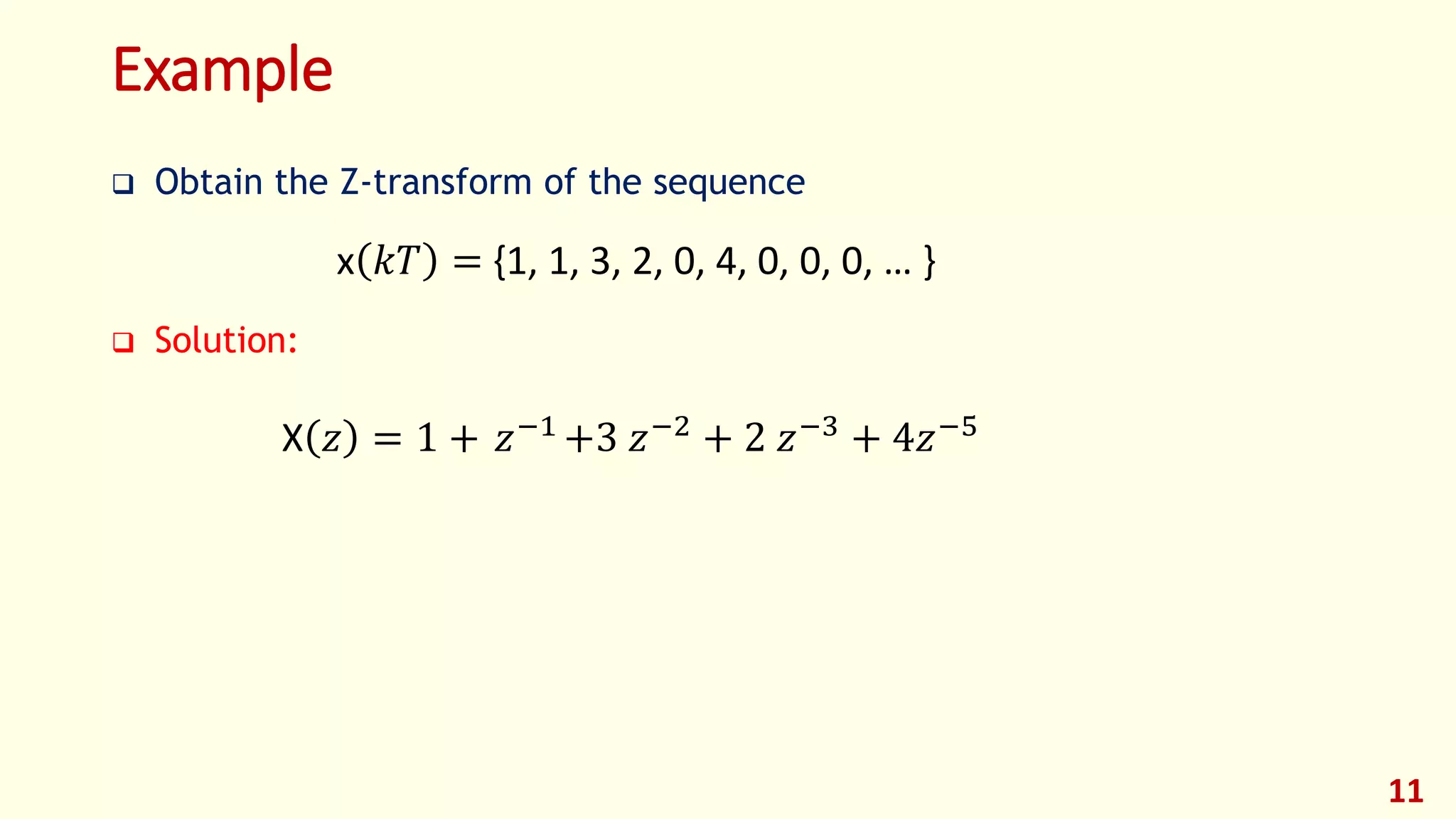
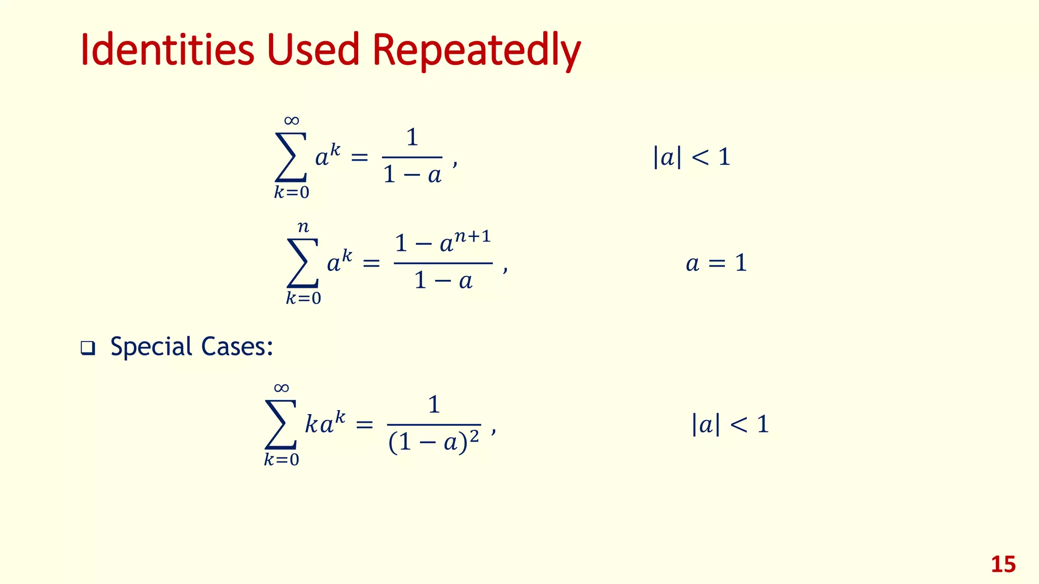
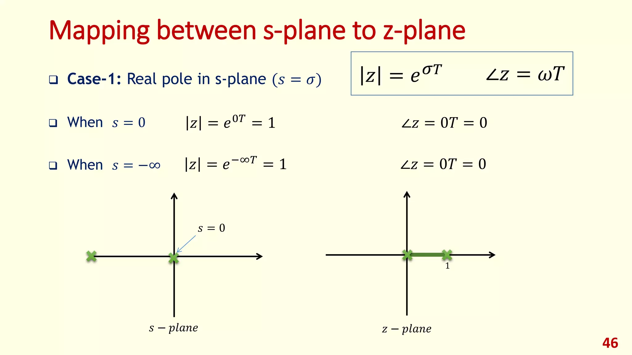
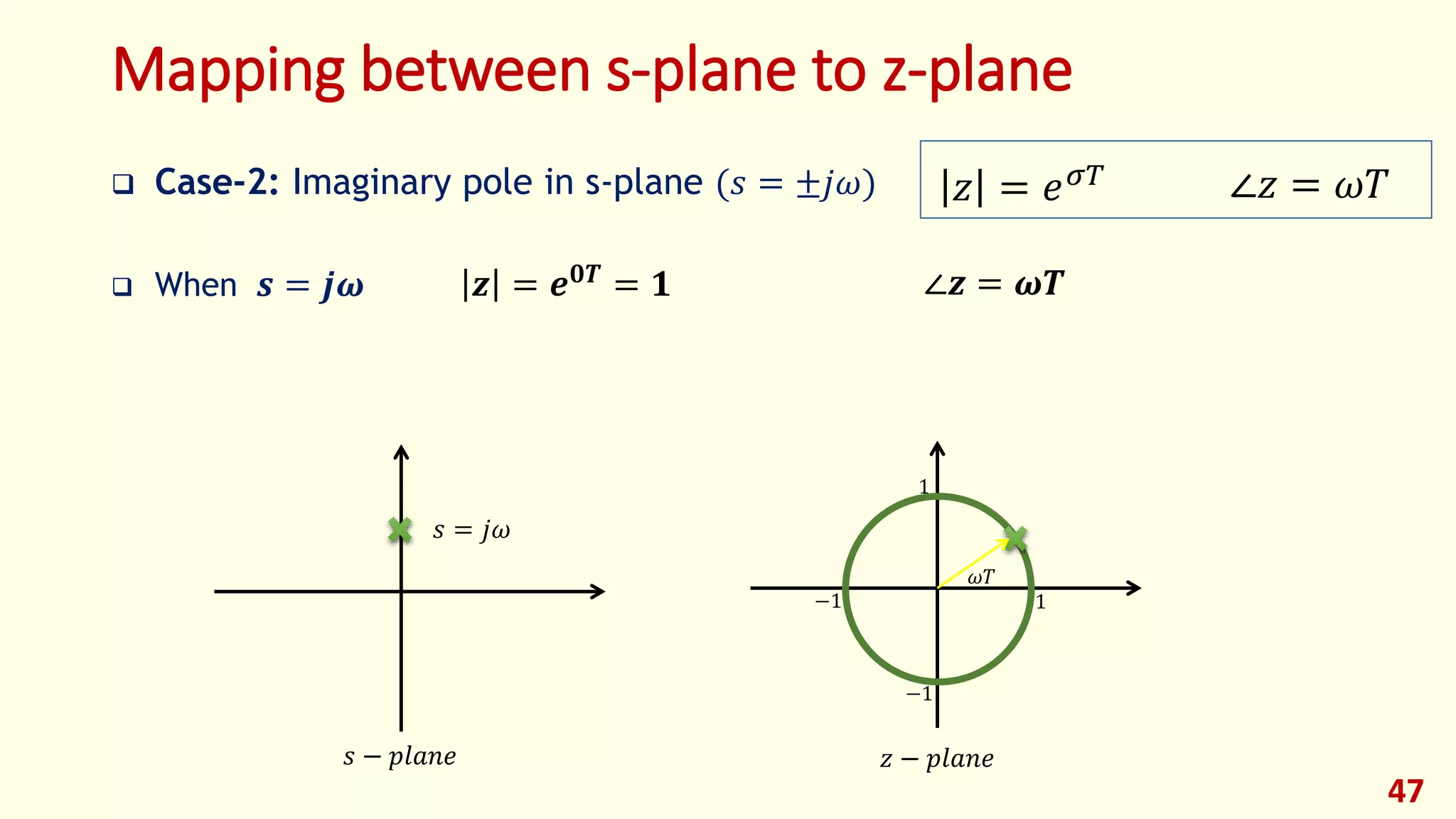
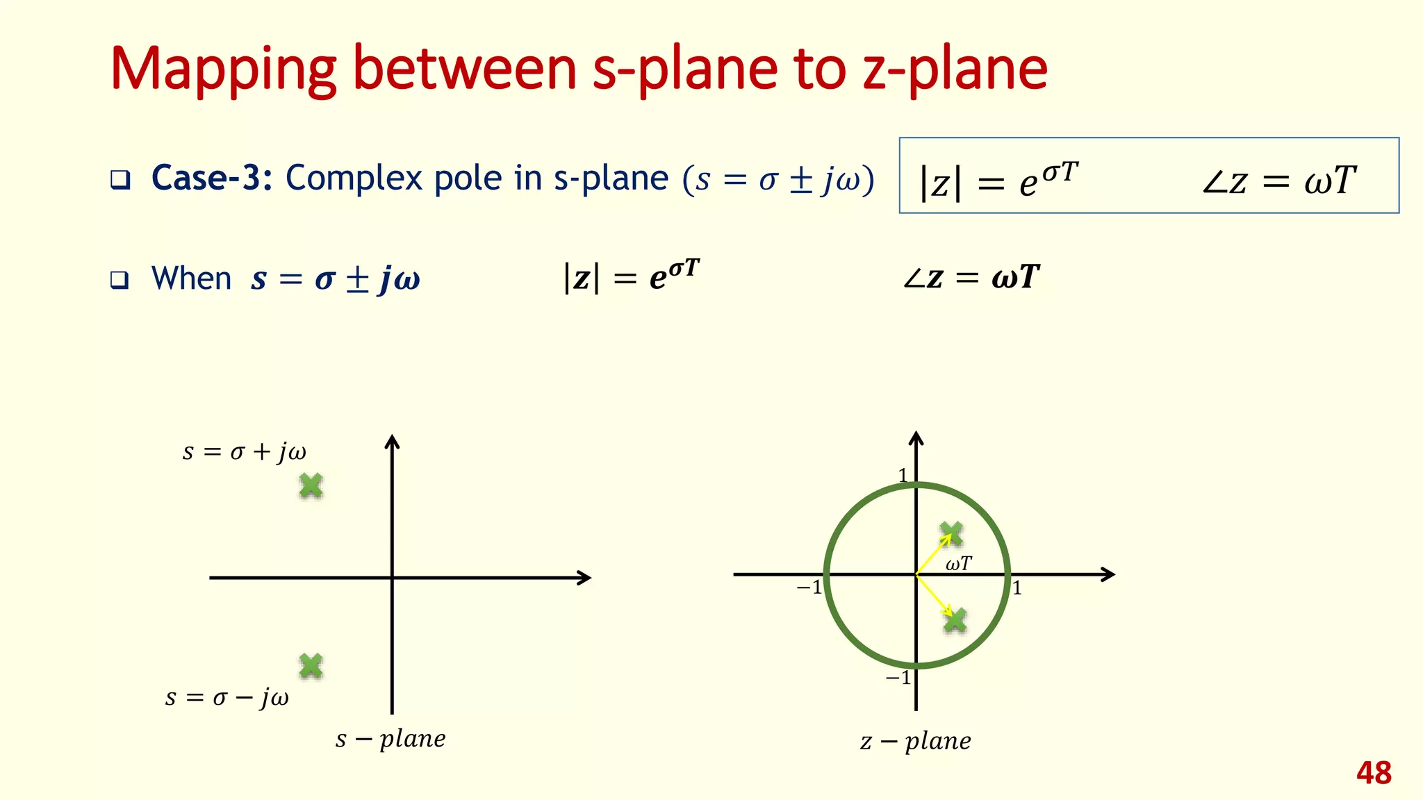
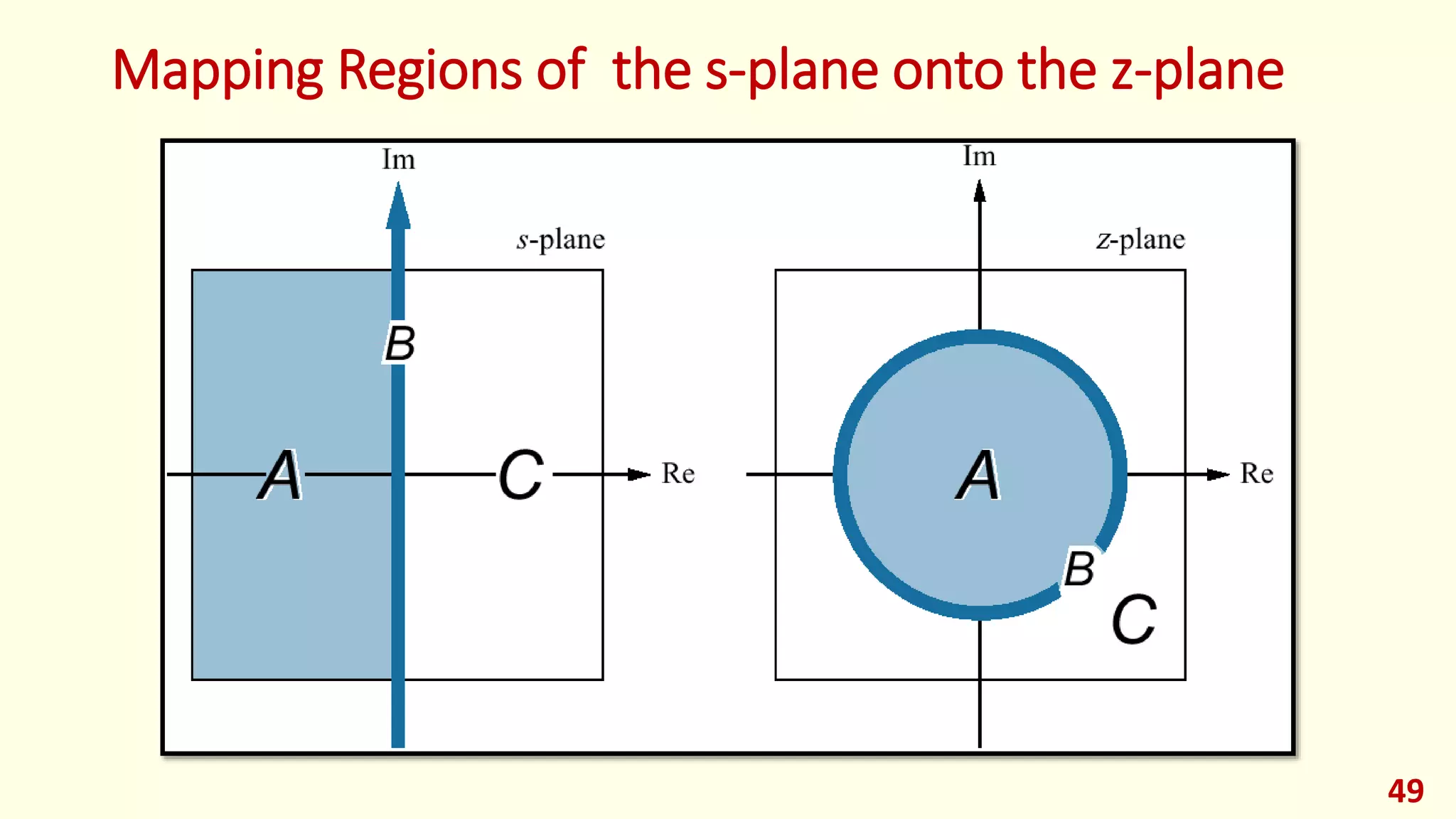
![Mapping between s-plane to z-plane
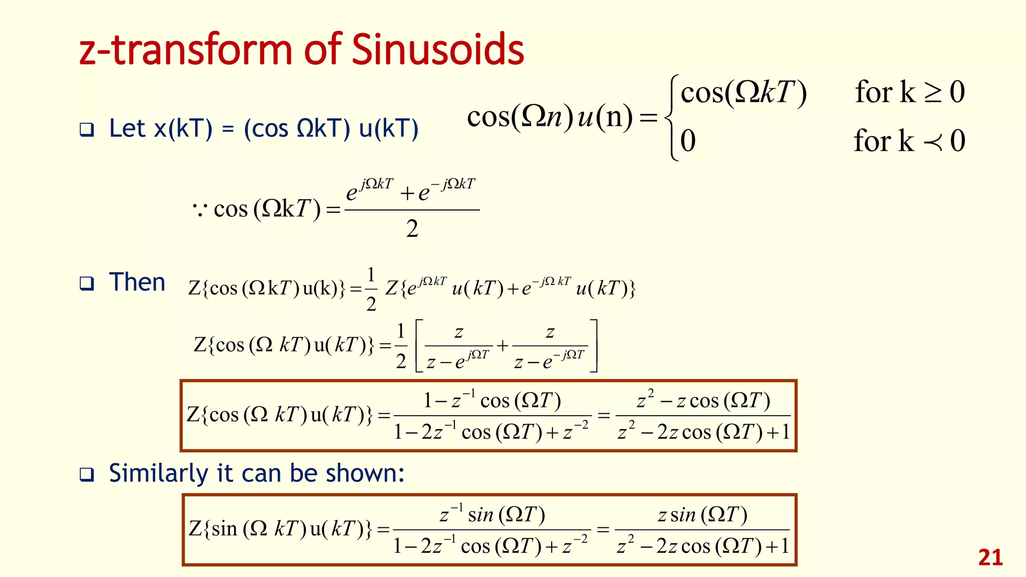
We will discuss following cases to map given points on s-plane to z-
plane.
Case-1: Real pole in s-plane (𝑠 = 𝜎) [on the left hand-side]
Case-2: Imaginary Pole in s-plane (𝑠 = 𝑗𝜔)
Case-3: Complex Poles (𝑠 = 𝜎 + 𝑗𝜔)
45𝑠 − 𝑝𝑙𝑎𝑛𝑒 𝑧 − 𝑝𝑙𝑎𝑛𝑒](https://image.slidesharecdn.com/dcs-lec02-z-transform-191118221227/75/Dcs-lec02-z-transform-45-2048.jpg)

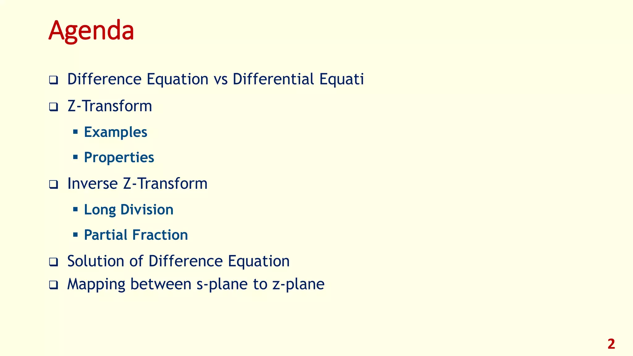
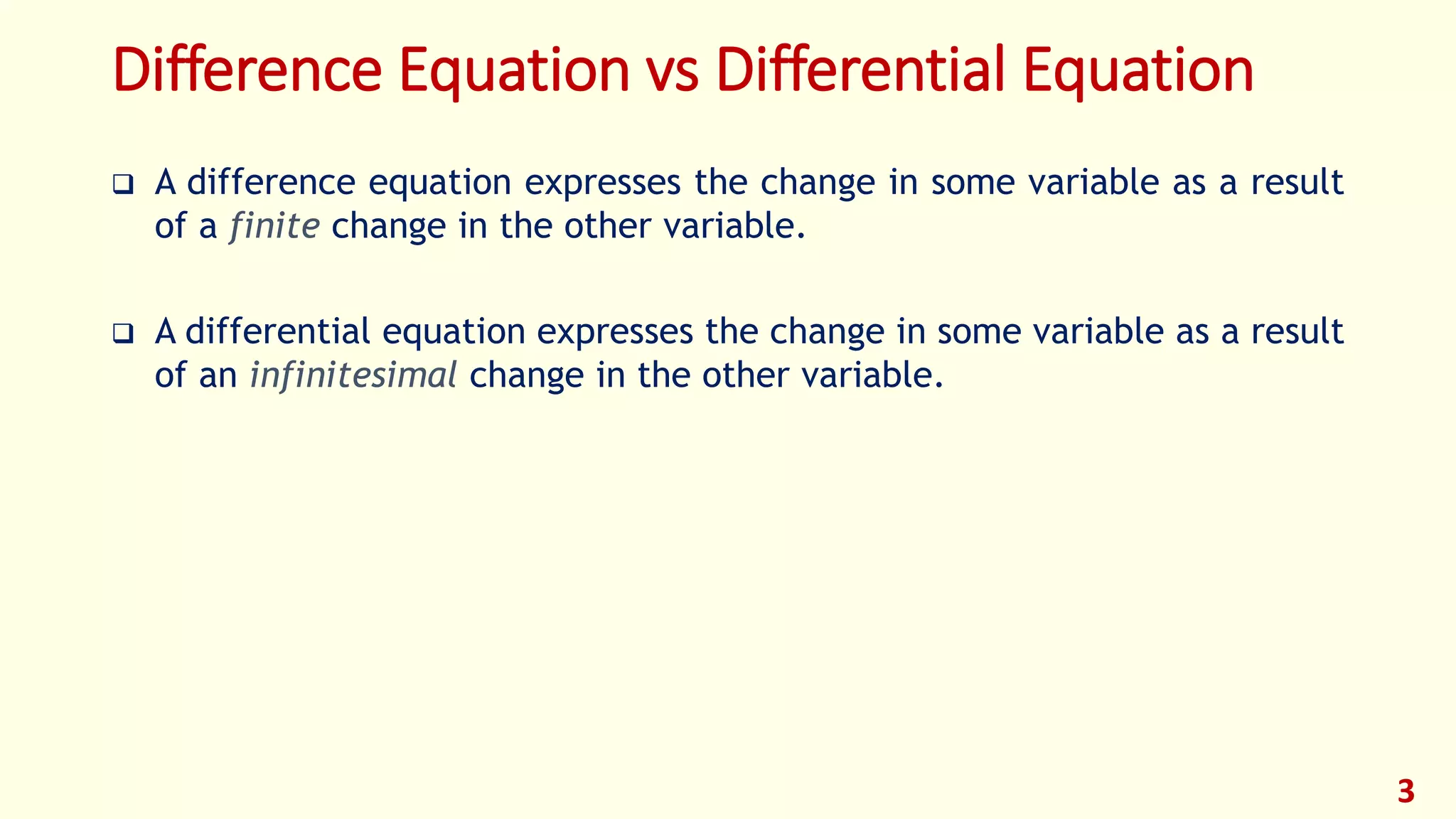
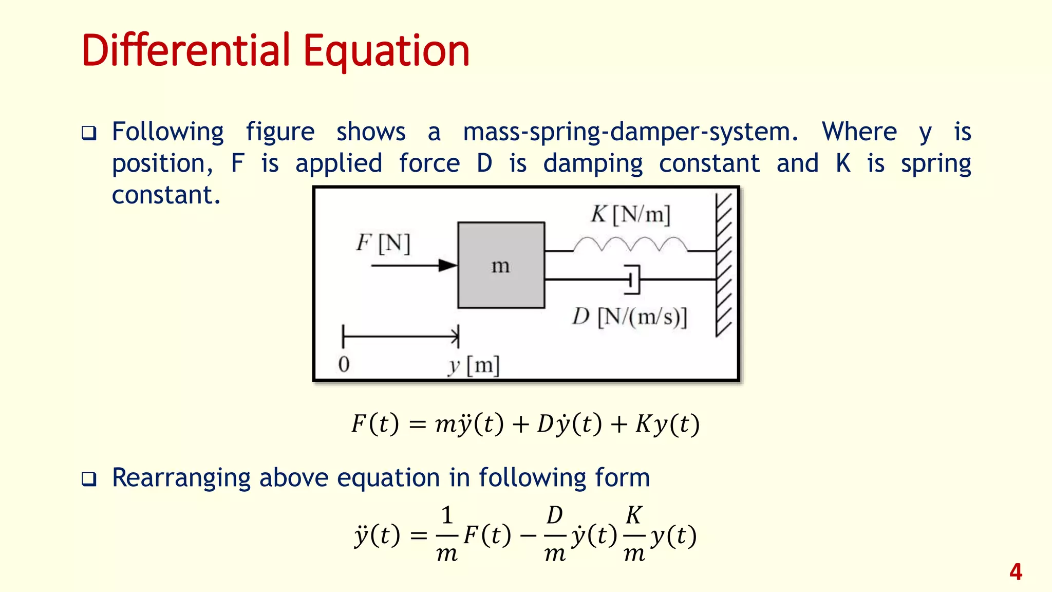
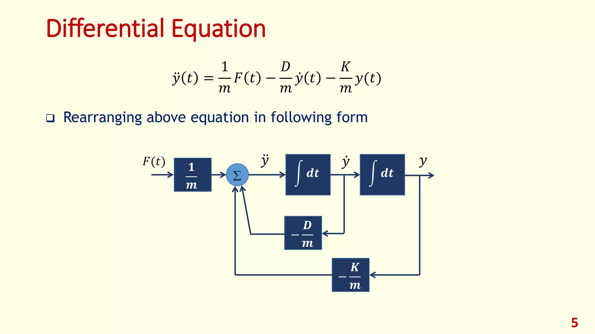
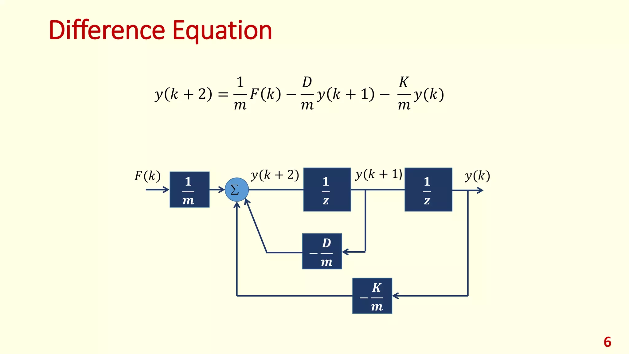
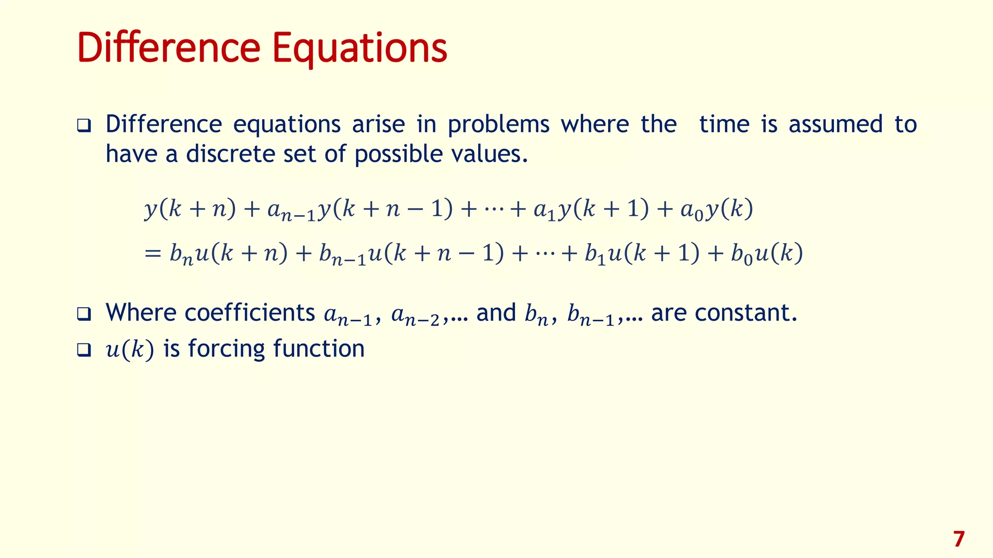
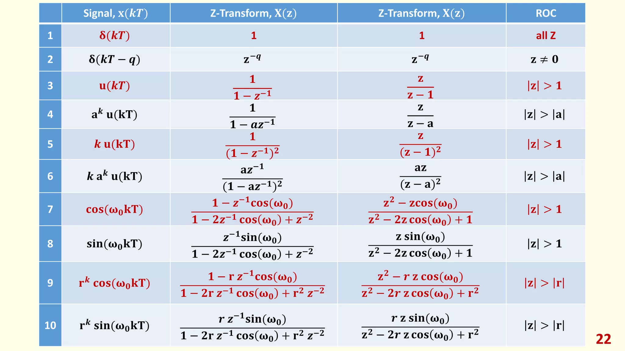
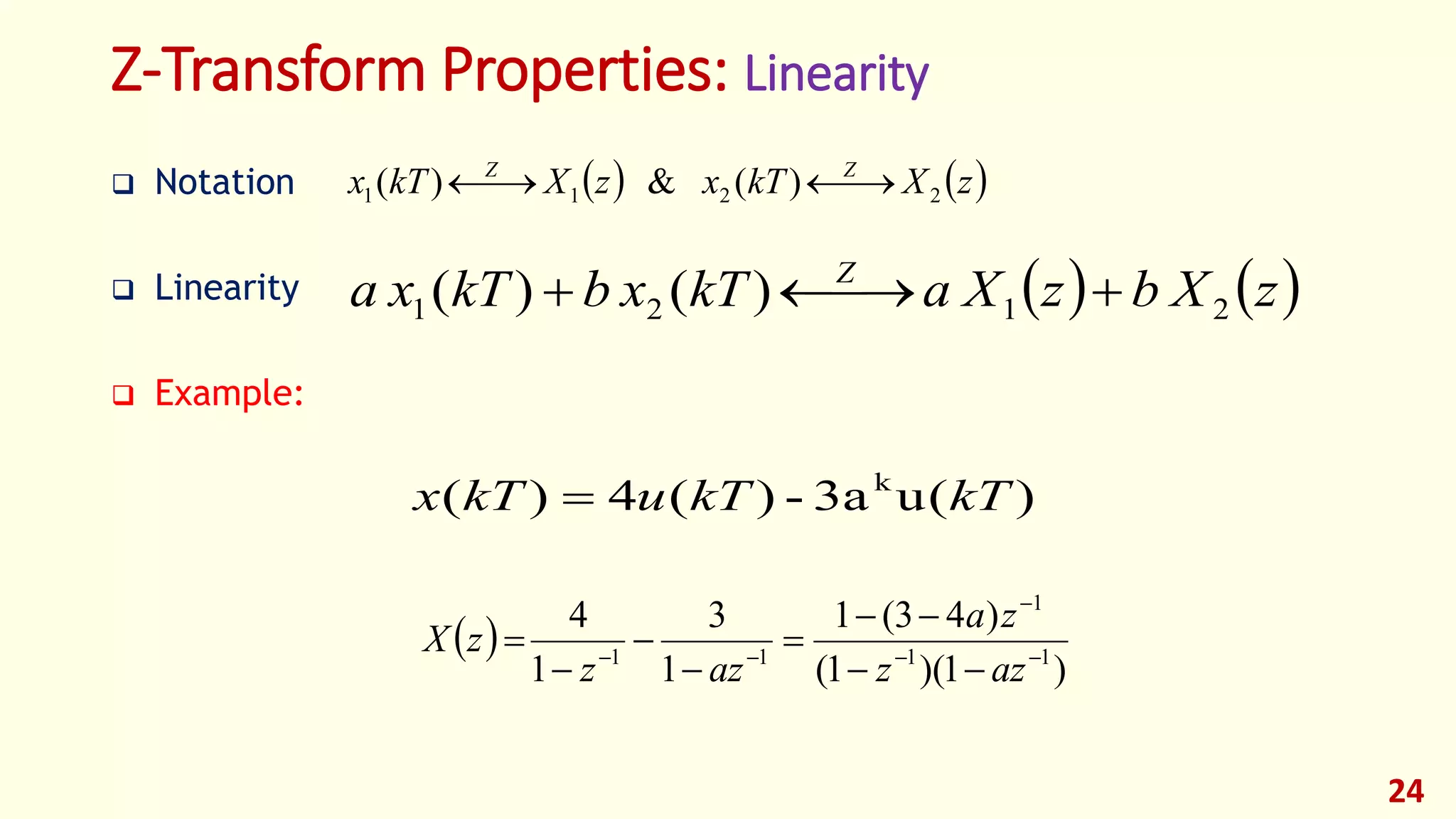
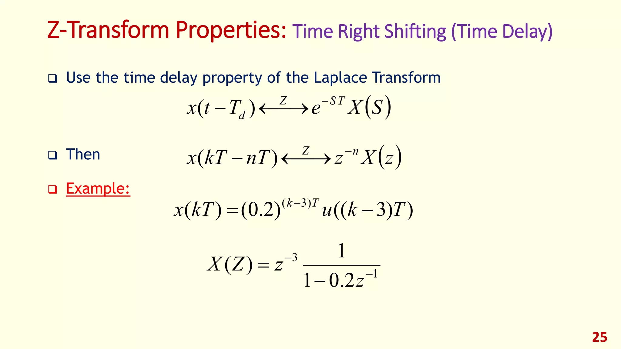
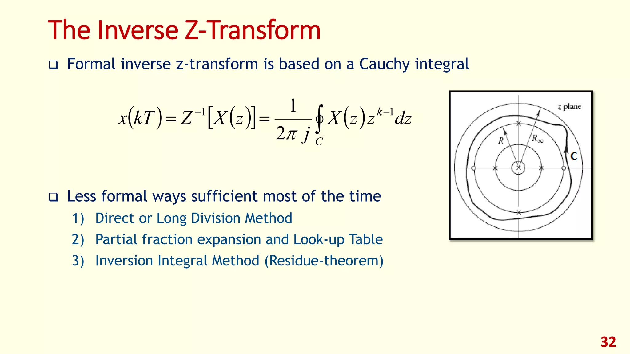
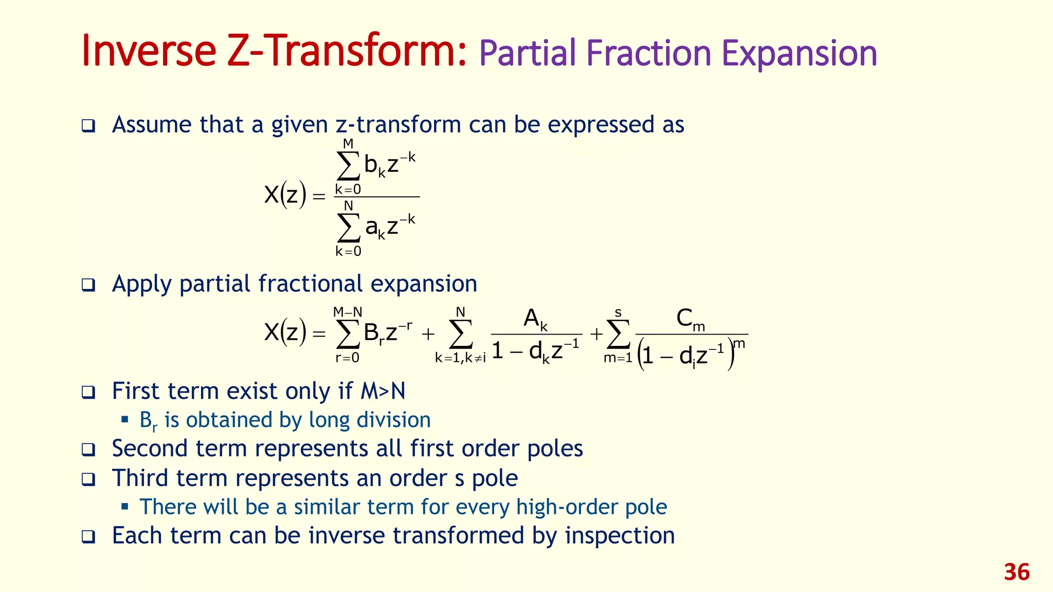
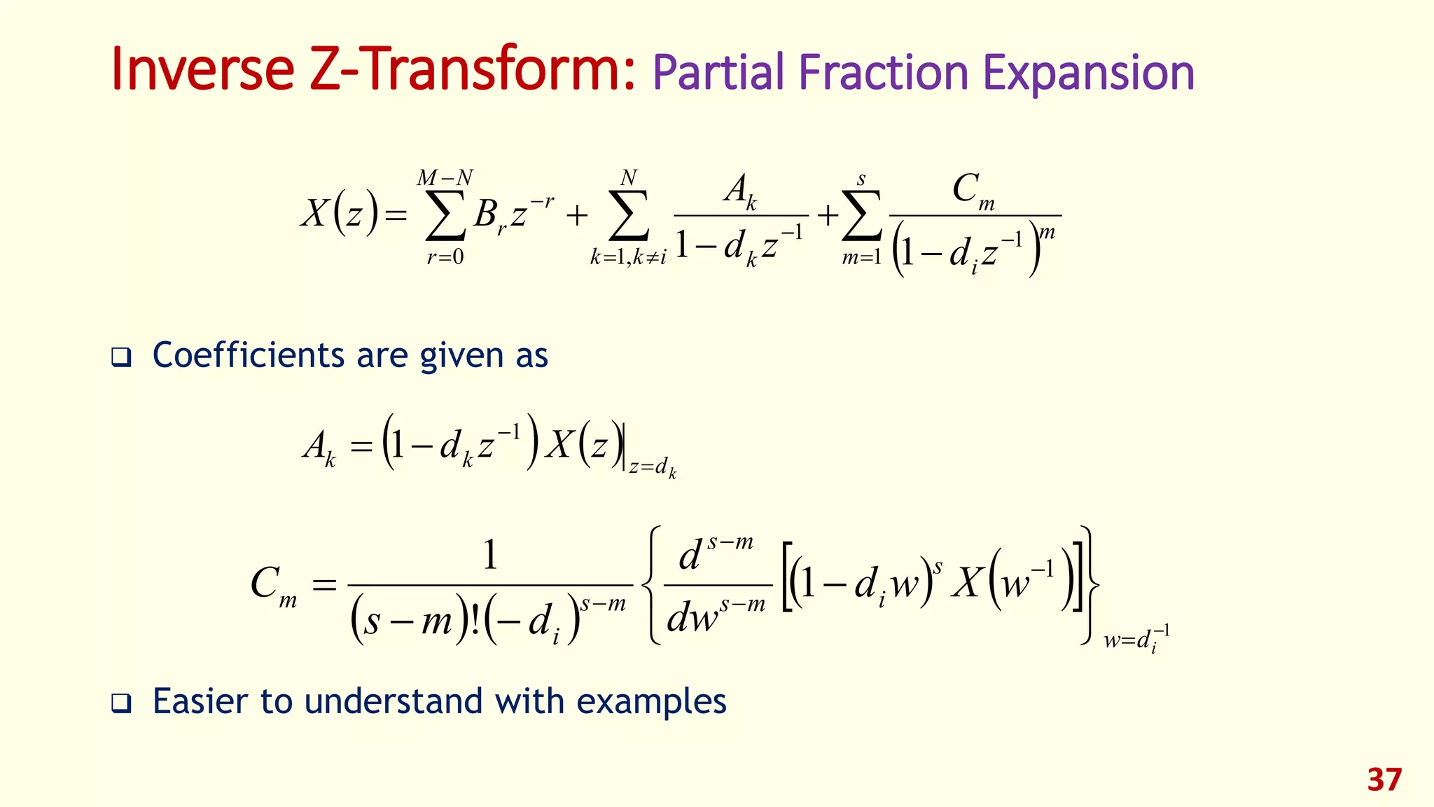
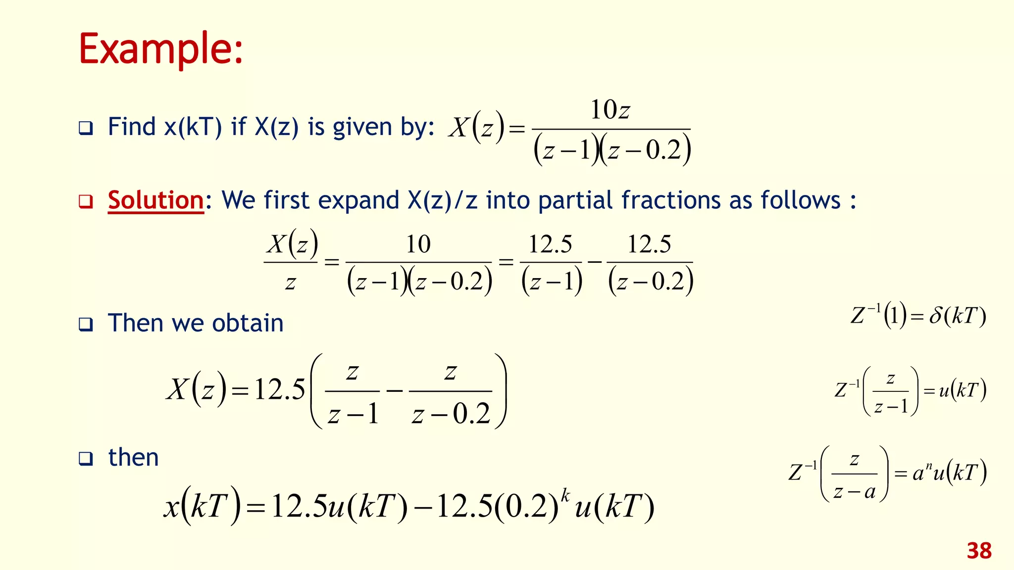
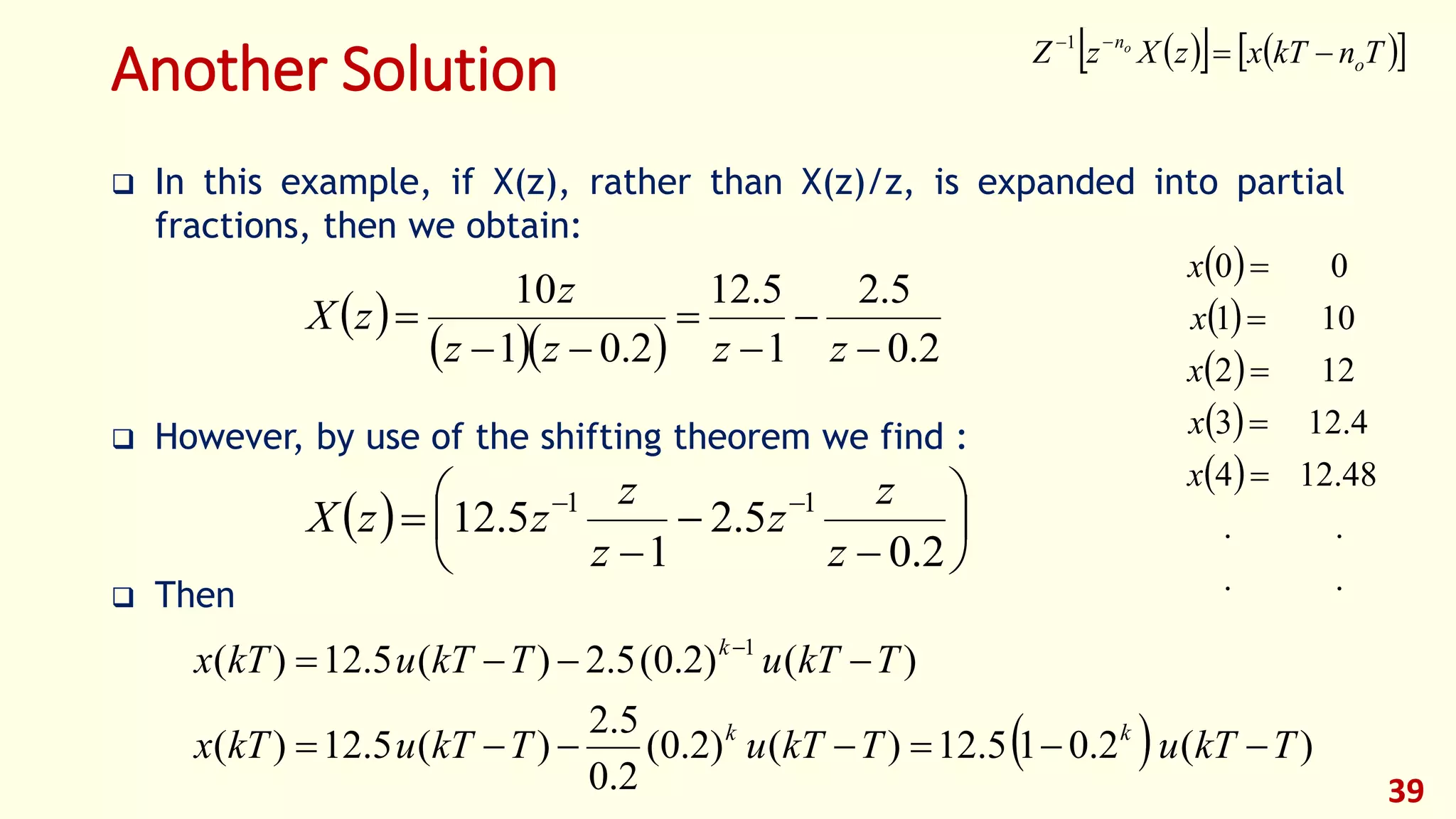
The document discusses the Z-transform, which is a tool for analyzing and solving linear time-invariant difference equations. It defines the Z-transform, provides examples of common sequences and their corresponding Z-transforms, and discusses properties such as the region of convergence. Key topics covered include the difference between difference and differential equations, properties of linear time-invariant systems, and mapping between the s-plane and z-plane.