Download as PDF, PPTX

![Multi-channel & Multidimensional Signals
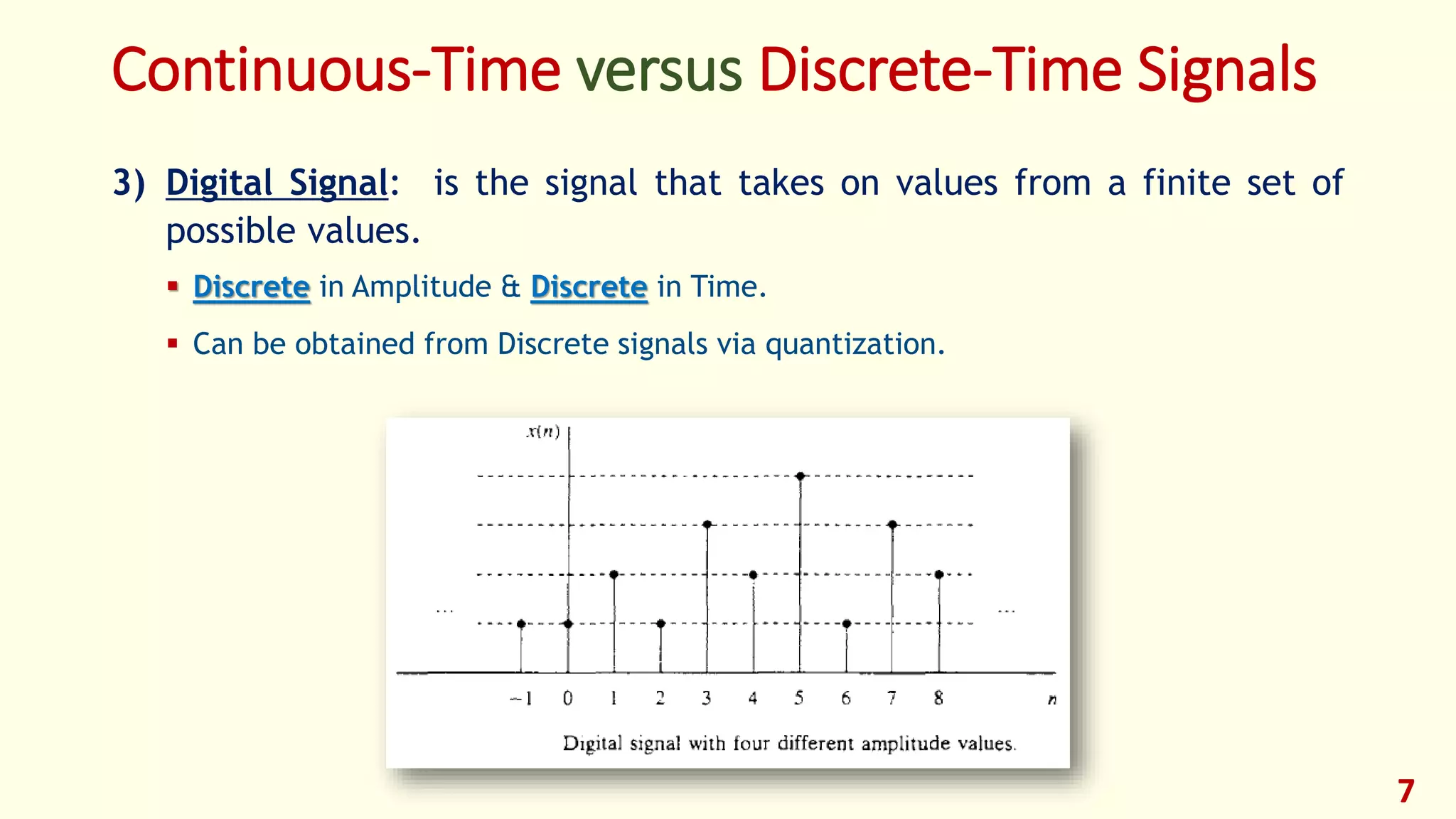
2) Multidimensional Signals:
If the signal is a function of a single independent variable, the signal called a
one-dimensional signal.
On the other hand , a signal called M-dimensional if its value is a function of M
independent variables.
The gray picture is an example of a 2-dimensional signal, the brightness or the
intensity I(x,y) at each point is a function of 2 independent variables.
The black & white TV picture [I(x,y,t)]: is a “3-Dimensional” since the
brightness is a function of time.
The color TV picture: is a multi-channel/multidimensional signal.
),,(
),,(
),,(
),,(
tyxI
tyxI
tyxI
tyxI
b
g
r
15](https://image.slidesharecdn.com/dsp2018foehu-lec1-introductiontodigitalsignalprocessing-180211195705/75/DSP_2018_FOEHU-Lec-1-Introduction-to-Digital-Signal-Processing-15-2048.jpg)
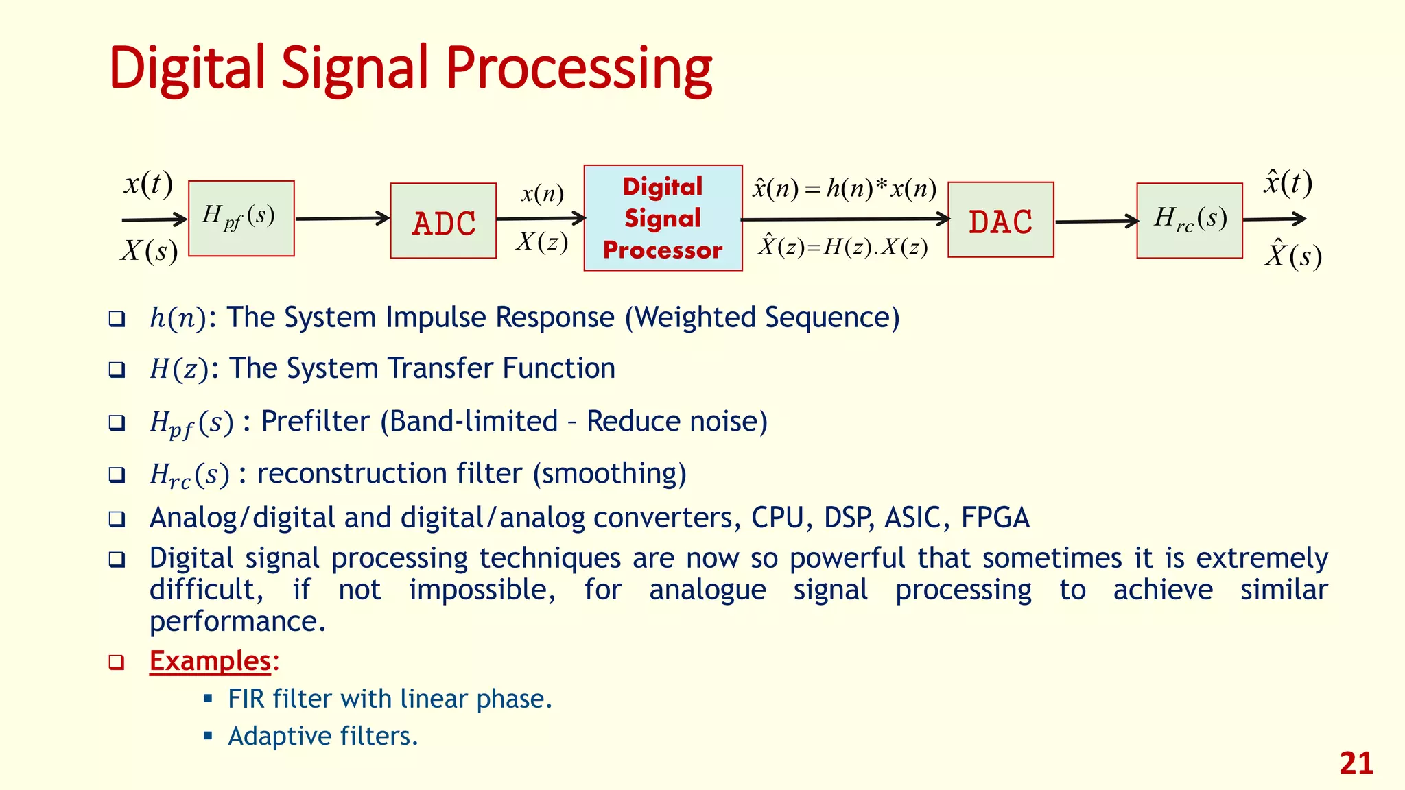


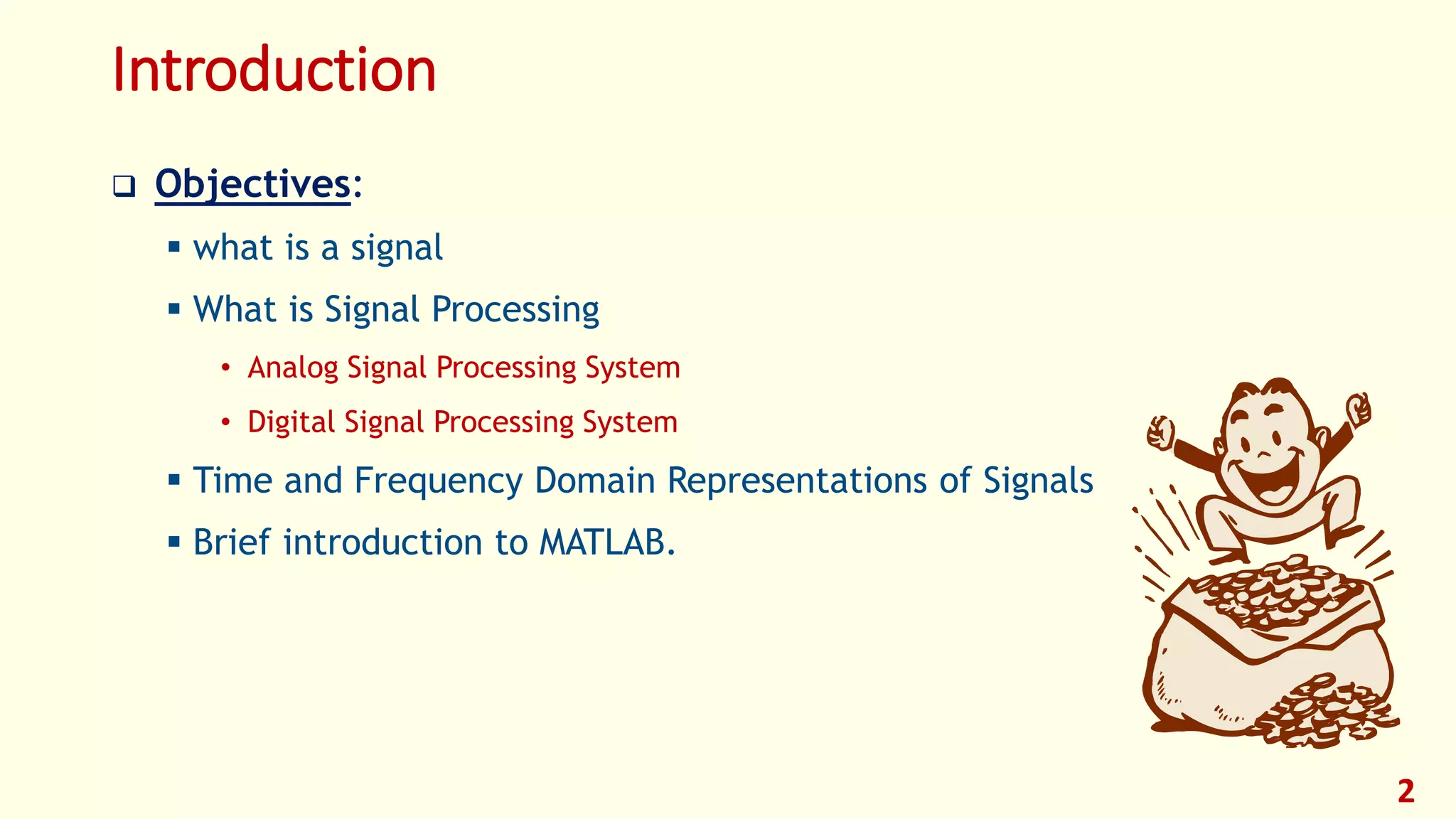
This lecture provides an introduction to digital signal processing. It defines what a signal is and discusses different types of signals including analog, discrete-time, and digital signals. It also covers signal classifications such as deterministic vs random, stationary vs non-stationary, and finite vs infinite length signals. The lecture then discusses analog signal processing systems and digital signal processing systems as well as transformations between time and frequency domains. It provides an overview of pros and cons of analog vs digital signal processing and examples of applications of digital signal processing.


![Digital Signal Processing[ECEG-3171]-Ch1_L03](https://cdn.slidesharecdn.com/ss_thumbnails/dspl3-180427094423-thumbnail.jpg?width=640&height=640&fit=bounds)


![Digital Signal Processing[ECEG-3171]-Ch1_L02](https://cdn.slidesharecdn.com/ss_thumbnails/dspl2-180427094423-thumbnail.jpg?width=640&height=640&fit=bounds)