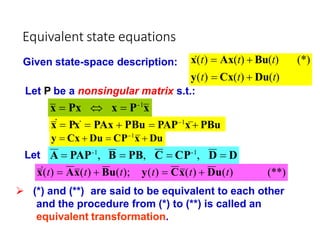
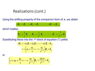
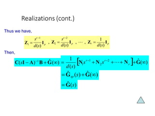
INSPIRING CREATIVE AND INNOVATIVE MINDS
State-Space Realizations
Example 3.1
Consider:
x
(t)  Ax(t)  Bu(t)
y(t)  Cx(t)  Du(t)
x
(t)  Ax(t)  Bu(t)
y(t)  Cx(t)  Du(t)
x(t)  Px(t)
Equivalent
Transformation
Equivalent
Systems
Equivalent state equations
Given state-space description:
Let P be a nonsingular matrix s.t.:
x  Px  x  P-1
x
x
 Px  PAx  PBu  PAP1
x  PBu
y  Cx  Du  CP1
x  Du
A  PAP-1
, B  PB, C  CP-1
, D  D
x
(t)  Ax(t)  Bu(t); y(t)  Cx(t)  Du(t) (**)
 (*) and (**) are said to be equivalent to each other
and the procedure from (*) to (**) is called an
equivalent transformation.
x
(t)  Ax(t)  Bu(t) (*)
y(t)  Cx(t)  Du(t)
Let
()  I  A
The feedforward matrix D between the input and output has nothing
to do with the state space and is not affected by the equivalent
transformation.
The characteristic equation for (*) is:
For (**), we have
()  I  A  I P1
AP  P1
P P1
AP
 P1
(λI)P P1
AP  P1
(λI  A)P
 P P1
λI  A  I A
Equivalent state equations have the same characteristic polynomial
and hence the same set of eigenvalues.
Equivalent state equations
Recall: A  PAP-1
and A are similar to each other
 They have same eigenvalues, same stability perf.
 Similar transfer functions!!
G(s)  C(sI  A)1
B  D G(s)  C(sI  A)1
B  D
and
G(s)  G(s)
To verify,
G(s)  C(sI  A)1
B  D
(XYZ)1
 Z1
Y1
X1
 CP-1
(sPP1
 PAP1
)1
PB  D
 CP-1
(P(sI - A)P-1
)-1
PB  D
 CP1
P(sI  A)1
P1
PB  D
 C(sI  A)1
B  D  G(s)
Equivalent state equations
Example 3.2
Consider again Ex. 3.1:
x1  x1
 2    2 
1x 
0 x1 
x  1
x1 

1
x(t)  Px(t)
From the circuit (via observation):
x2  (x1  x2 )1
Or
 
 
   
1
1
1
1 1
1 0
x2 
x 
x2 
x 
  
1
 
1
1
1x2 
0 x 
Two state equations are said to be zero-state equivalent
if they have the same transfer matrix or
D  C(sI  A)1
B  D  C(sI  A)1
B
Note that:
(sI  A)1
 s1
I  s2
A s3
A2

Then,
D  CBs1
 CABs2
 CA2
Bs3
 D  CBs1
 CABs2
 CA2
Bs3

Zero-State Equivalent
matrix iff
Theorem 3.1
Two LTI state equations{A,B,C,D} and {A,B, C, D}
are zero-state equivalent or have the same transfer
D  D and
CAm
B  CAm
B ; m  0,1,2,...
- In order for two state equations to be equivalent, they
must have the same dimension.
- This is, however, not the case for zero-state equivalence.
Example 3.3:
Consider:
A  B  C  0
y(t)  0.5u(t) x(t)  x(t)
y(t)  0.5x(t)  0.5u(t)
A 1 ; B  0 ; C  0.5 ; D  0.5
D  D  0.5
CAm
B  CAm
B  0
Note that:
 The two systems are zero-state equivalent.~ Theorem 3.1
Companion Form
• Consider:
0
 3 2 1
 1 0 x(t)  0u(t)  Ax(t)  bu(t)
  
 4 3 1  1
x
(t)   2
• Then:
• It can be shown that:
• Can {b,Ab,A2
b} be used as the basis?
 YES!
Companion Form

5 


0
0 0 17 
0 15
1
A  1
• Then:
• Thus the representation ofA w.r.t. the basis {b,Ab,A2
b} is:
Companion Form


 0


0

0 
0 
 1
;

0
1
1  
 
3

 0
2   0 1
0
0 0 0 4  1 2 3 4 
 0 0 0
0 1 0 0
0 1 1


 0
0
;

1 

 0
0 
 0
 4
2
1
2
3
4

 0 1 0 0  1 1 0 0
0 1 0 1 
0 0 3 0 0 1
0 0
     
Transpose
All have similar
characteristic
polynomial:
2 3 4
1
4 3 2
()         
• Companion-form matrices:
• Any special?
 3
52
15 17  0
( 3)  2 1
2 ( 1) 0
 4 3 ( 1)
()  I  A 
A  1
(-1)
(-1)
0 0 17 
 0 15

0 1 5 

(-1)
Realizations
Q. What is "realization"?
space equation
– Implicitly implies LTI systems
– Shall start with multi-variable systems and will
sometimes specialize to single-variable systems
x
(t)  Ax(t)  Bu(t)
y(t)  Cx(t)  Du(t)
D(s)
– For a givenĜ(s) 
N(s)
, find a corresponding state-
Q. If Ĝ(s) is realizable, how many possible
realizations?
– Infinite ~ in view of equivalent transformations and the
possibility of adding un-controllable or un-observable
components
Q. Which one is the "good" realization?
- A “good” realization is the one with the minimal order
~ Irreducible realization
 Will be discussed in Topic 6
Realizations (cont.)
Q. Under what condition is Ĝ(s) realizable by an
LTI system?
-Recall that the transfer function of the dynamic equation is
Ĝ(s)  C(sI  A)1
B  D  C(sI  A)1
B  D
Ĝ(s) is realizable by a dynamic equation iff it is a
proper rational function (order of numerator  order of
denominator)
 In fact, the part contributed by C(sI - A)-1B is
strictly proper
Theorem 3.2
Realizations (cont.)
as:
Ĝ
sI  A
(s) : C(sI  A)1
B 
1
CAdj.(sI  A)B
sp
To determine the realization of Ĝ(s) , decompose it
Ĝ(s)  Ĝ()Ĝsp (s)
where
r r1
1
d(s)  s  s  r1s r
Let
i.e. least common denominator of all entries of Ĝsp (s).
Nr 1
y  N1 N2  Nr xĜ()u
 
 0 
 

0 

x   0 u













0

0
x
 
Ip 
p
Realizations (cont.)
~Block companion form
1Ip 2I p  r1Ip rIp 
 I 0  0 0 
Ip  0 0
  
0  Ip 0
(rprp) (rpp)
(q rp)
where Ip is the p p unit matrix and every 0 is a p p zero matrix.
Then the realization of Ĝ(s) is given by
Realizations (cont.)
Proof:
Define,
Z1 
Z 
Z :  2  : (sI  A)1
B

Z

 r 
   i
where Z is the (pp) and Z is a (rpp).
Simplifying,
Then,
(sI  A)Z  B  sZ  AZ B (*)
 
  







 


0 

Z   0 
0
   
 

 0
0

0



Ip 
Zr


p
sZr


sZ 
0 Z3    0 
2 
sZ3   
2 
sZ1  rIp Z1 
1Ip 2I p  r1Ip
 I 0  0
Ip  0
 
0 Ip
Realizations (cont.)
Using the shifting property of the companion form of A, we obtain
Substituting these into the 1st block of equation (*) yields
which implies
 Zr 1
sZ2  Z1 , sZ3  Z2 ,  , sZr
sZ1  1Z1 2Z2 rZr Ip
1
3
2 1 Z
1 r
1
sr 1
s2
s
Z 
1
Z , Z 
1
Z ,  , Z 
p
r
s
s





1
r1
2
1
 
     Z I
or
p
r
s
s





sr 1
1
r1
2
1
 Z 
d(s)
 I

s   
Realizations (cont.)
Thus we have,
Then,
ˆ
1
2
1
C(sI  A)1
B  Ĝ()  G()
r
r2
r1
 N s
Ns
d(s)
 N
1
Z1 
d(s)
Ip
sr 2
sr 1
, Z2 
d(s)
Ip ,  , Zr 
d(s)
Ip
 Ĝsp (s)Ĝ()
 Ĝ(s)
Special Case: p = 1
Realizations (cont.)
(For simplicity, let r = 4 and q =2.)
Then, the realization is
Consider a 21 proper rational matrix:



22 23
3
 21 24 
14

13
2
12
3
11
4
3
2
1 2
4 3
2
ˆ
 s   s2
  s  
s  
s  
 s  
s  s 
s  s 
d 
d1  1
G(s)    
d 
 2 
24 
23
22
 21
 
 

14 
x 
d1 
u
y 
11 12 13
  0
1
0  0
0   
 0
 0
0  0
x   u
1 2 3 4 
 1 0 0
1 0
0 1
x
 
Note: The
controllable-
canonical-form
realization can be
read out from the
coefficients of Ĝ(s).
Realizations (cont.)
• A multi-input LTI system is the sum of many single-input
LTI systems, so can realize each single-input subsystem
and form the sum:
1st and 2nd column of




 
3
12
0 0
0



2
(s  2)2


s 1 
(2s1)(s  2)
s  2 
2s 1
1
 Ĝ()Ĝsp (s)
Example 3.3:
3




(s  2)2



s 1 
(2s1)(s  2)
s  2 
,
4s 10
2s 1
1
Ĝ(s) 

Consider a proper rational matrix

 

  

(2s 1)(s  2) (s  2)2


s  2 
2s 1
1 s 1
4s 10 3
Ĝ(s) 

Determine a realization of this transfer matrix.
Solution:
Decompose Ĝ(s) into a strictly proper rational matrix
d(s)  (s 0.5)(s  2)2
 s3
 4.5s2
6s  2
The monic least common denominator of Ĝsp (s) is




1
ˆ
(s 1)(s0.5) 
0.5(s 2)
3(s 2)(s 0.5)
6(s 2)2
s3
4.5s2
6s 2
sp
G
Example (cont.)
Thus



 2
(s 1.5s 0.5)
3(s2
2.5s1) 
1 6(s2
4s 4)
d(s)  0.5(s 2)


 2
s 1.5s 0.5
3s2
7.5s3
1 6s2
24s 24
d(s)  0.5s 1

 
 


0.5
1.5  1
 0.5
24
 6 3
1 2
7.5
s
24 3 
s 
d(s)  0 1
 
 
 
  2 
1
0.5
 0 0 0u 
2 0 u
x
y 
6
Example (cont.)
Given,
 


  
  

 0 0
0 1
0 1 0 0
0 0 1 0 0 

0
0
0
1


 1
0
0 6 0 2 0  1 0
0 4.5 0 6 0 2
4.5
0u2 
0 0 0 0  0 0u1 
0 0 0 0  0
 
0  0 0
x
x
 



3




(s  2)2



s 1 
(2s1)(s  2)
s  2 
,
4s 10
2s 1
1
Ĝ(s) 

A B
3 24 7.5 24 3
1 0.5 C
1.5 1 D
Ĝ(s)
 A,B,C,D
B


C D
S 
A
Realization
the realization is,
Example 3.4:



 


(2s1)(s  2)

4s 10
2s 1
1

(s) 
c1
Ĝ
The 1st column is
Consider again the proper rational matrix in Ex. 3.3.





 3
(s  2)2


s 1
(2s 1)(s  2)
s  2 
4s 10
2s 1
1
Ĝ(s) 

1
 

 (2s 1)(s 2) 

(4s 10)(s  2)

 

 
 (2s 1)(s 2) 
   
1
2

2s2
5s 2 

2s 5s 2
4s2
2s 20
In Matlab: n1=[4 -2 -20;0 0 1]; d1=[2 5 2]; [a,b,c,d]=tf2ss(n1,d1)
Ex. 3.4 (cont.)
Using MATLAB: n1=[4 -2 -20;0 0 1];d1=[2 5 2];[a,b,c,d]=tf2ss(n1,d1)
yields the following realization for the 1st column of Ĝ(s):
1
1
1
c1 1 1 1 1 0
0.5 
 0
   
0  1 0 1
  
1 1 1 1 1 

12
x 
2
u
y  C x d u 
6
1
x 
1
u
x
  A x b u 
2.5
Similarly, the function tf2ss can generate the following realization for the
2nd column of Ĝ(s):
2
2
2
2
2 2 2 2 2
c2 2 2 2 2 0
1 1
   
  
 1 0  0

6
x 
0
u
y C x d u 
3
4
x 
1
u
x
  A x b u 
4
Example 3.4 (cont.)
Notice that:





 3
(s  2)2


s 1

(2s 1)(s  2)
s  2 
2s 1
1
4s 10
Ĝ(s) 

Ex. 3.4 (cont.)
 2   2  2   2  2 
x   0 A x   0 b u 
These two realizations can be combined as
x1

A1 0 x1 

b1 0 u1 
y  yc1 yc2  C1 C2 xd1 d2 u
or
u





 
x

 




x u
0 0
y   0
6 12 3 6 2 0
1
0 1
0 0 4 4
0 0 
0  0 0
0
1
1 0 0  1 0
0
2.5
x
  

 

 










2 

0
0 1
0  0 0
0  0
1
0
2
0  1 0
0 6 0 2
0 4.5 0 6 0
 4.5
0u 
0 0 0 0 0  0
x
1 0 0 0
x

 



  2 
0.5
 0
0 0 1 0 0
 
0 0 0 1 0 0 0
3 24 7.5 24
1 0.5 1.5 1 u


0u1 
3 
x 
2
y 
6
A
(4
0x4)
1
B
(

4
0x20)
0
C
.5 1
(2x4)
 
D
(2x2)
A
(6x6)
B0u1
(6x2)
C
(2x6)
0
D
0
(2x2)
Example 3.4 (cont.)
• Can also focus on the realizations of single-output systems. Then treat
LTI systems with multi-outputs as combinations of single-outputs
subsystems.
• i-th row of
• Overall realization:

0

0
  
cq

 dq


  
Aq

 Bq


x    u
x
 
Realize with {Ai, Bi, ci, di}
c1 0  d1 
0  B1 
A1
 x    u ;y   

State Space Realizations_new.pptx

  • 1.
    INSPIRING CREATIVE ANDINNOVATIVE MINDS State-Space Realizations
  • 2.
    Example 3.1 Consider: x (t) Ax(t)  Bu(t) y(t)  Cx(t)  Du(t) x (t)  Ax(t)  Bu(t) y(t)  Cx(t)  Du(t) x(t)  Px(t) Equivalent Transformation Equivalent Systems
  • 3.
    Equivalent state equations Givenstate-space description: Let P be a nonsingular matrix s.t.: x  Px  x  P-1 x x  Px  PAx  PBu  PAP1 x  PBu y  Cx  Du  CP1 x  Du A  PAP-1 , B  PB, C  CP-1 , D  D x (t)  Ax(t)  Bu(t); y(t)  Cx(t)  Du(t) (**)  (*) and (**) are said to be equivalent to each other and the procedure from (*) to (**) is called an equivalent transformation. x (t)  Ax(t)  Bu(t) (*) y(t)  Cx(t)  Du(t) Let
  • 4.
    ()  I A The feedforward matrix D between the input and output has nothing to do with the state space and is not affected by the equivalent transformation. The characteristic equation for (*) is: For (**), we have ()  I  A  I P1 AP  P1 P P1 AP  P1 (λI)P P1 AP  P1 (λI  A)P  P P1 λI  A  I A Equivalent state equations have the same characteristic polynomial and hence the same set of eigenvalues. Equivalent state equations
  • 5.
    Recall: A PAP-1 and A are similar to each other  They have same eigenvalues, same stability perf.  Similar transfer functions!! G(s)  C(sI  A)1 B  D G(s)  C(sI  A)1 B  D and G(s)  G(s) To verify, G(s)  C(sI  A)1 B  D (XYZ)1  Z1 Y1 X1  CP-1 (sPP1  PAP1 )1 PB  D  CP-1 (P(sI - A)P-1 )-1 PB  D  CP1 P(sI  A)1 P1 PB  D  C(sI  A)1 B  D  G(s) Equivalent state equations
  • 6.
    Example 3.2 Consider againEx. 3.1: x1  x1  2    2  1x  0 x1  x  1 x1   1 x(t)  Px(t) From the circuit (via observation): x2  (x1  x2 )1 Or         1 1 1 1 1 1 0 x2  x  x2  x     1   1 1 1x2  0 x 
  • 7.
    Two state equationsare said to be zero-state equivalent if they have the same transfer matrix or D  C(sI  A)1 B  D  C(sI  A)1 B Note that: (sI  A)1  s1 I  s2 A s3 A2  Then, D  CBs1  CABs2  CA2 Bs3  D  CBs1  CABs2  CA2 Bs3  Zero-State Equivalent
  • 8.
    Zero-State Equivalent matrix iff Theorem3.1 Two LTI state equations{A,B,C,D} and {A,B, C, D} are zero-state equivalent or have the same transfer D  D and CAm B  CAm B ; m  0,1,2,... - In order for two state equations to be equivalent, they must have the same dimension. - This is, however, not the case for zero-state equivalence.
  • 9.
    Example 3.3: Consider: A B  C  0 y(t)  0.5u(t) x(t)  x(t) y(t)  0.5x(t)  0.5u(t) A 1 ; B  0 ; C  0.5 ; D  0.5 D  D  0.5 CAm B  CAm B  0 Note that:  The two systems are zero-state equivalent.~ Theorem 3.1
  • 10.
    Companion Form • Consider: 0 3 2 1  1 0 x(t)  0u(t)  Ax(t)  bu(t)     4 3 1  1 x (t)   2 • Then: • It can be shown that: • Can {b,Ab,A2 b} be used as the basis?  YES!
  • 11.
    Companion Form  5    0 00 17  0 15 1 A  1 • Then: • Thus the representation ofA w.r.t. the basis {b,Ab,A2 b} is:
  • 12.
    Companion Form    0   0  0 0   1 ;  0 1 1     3   0 2   0 1 0 0 0 0 4  1 2 3 4   0 0 0 0 1 0 0 0 1 1    0 0 ;  1    0 0   0  4 2 1 2 3 4   0 1 0 0  1 1 0 0 0 1 0 1  0 0 3 0 0 1 0 0       Transpose All have similar characteristic polynomial: 2 3 4 1 4 3 2 ()          • Companion-form matrices: • Any special?  3 52 15 17  0 ( 3)  2 1 2 ( 1) 0  4 3 ( 1) ()  I  A  A  1 (-1) (-1) 0 0 17   0 15  0 1 5   (-1)
  • 13.
    Realizations Q. What is"realization"? space equation – Implicitly implies LTI systems – Shall start with multi-variable systems and will sometimes specialize to single-variable systems x (t)  Ax(t)  Bu(t) y(t)  Cx(t)  Du(t) D(s) – For a givenĜ(s)  N(s) , find a corresponding state-
  • 14.
    Q. If Ĝ(s)is realizable, how many possible realizations? – Infinite ~ in view of equivalent transformations and the possibility of adding un-controllable or un-observable components Q. Which one is the "good" realization? - A “good” realization is the one with the minimal order ~ Irreducible realization  Will be discussed in Topic 6 Realizations (cont.)
  • 15.
    Realizations (cont.) Q. Underwhat condition is Ĝ(s) realizable by an LTI system? -Recall that the transfer function of the dynamic equation is Ĝ(s)  C(sI  A)1 B  D  C(sI  A)1 B  D Ĝ(s) is realizable by a dynamic equation iff it is a proper rational function (order of numerator  order of denominator)  In fact, the part contributed by C(sI - A)-1B is strictly proper Theorem 3.2
  • 16.
    Realizations (cont.) as: Ĝ sI A (s) : C(sI  A)1 B  1 CAdj.(sI  A)B sp To determine the realization of Ĝ(s) , decompose it Ĝ(s)  Ĝ()Ĝsp (s) where r r1 1 d(s)  s  s  r1s r Let i.e. least common denominator of all entries of Ĝsp (s).
  • 17.
    Nr 1 y N1 N2  Nr xĜ()u    0     0   x   0 u              0  0 x   Ip  p Realizations (cont.) ~Block companion form 1Ip 2I p  r1Ip rIp   I 0  0 0  Ip  0 0    0  Ip 0 (rprp) (rpp) (q rp) where Ip is the p p unit matrix and every 0 is a p p zero matrix. Then the realization of Ĝ(s) is given by
  • 18.
    Realizations (cont.) Proof: Define, Z1  Z Z :  2  : (sI  A)1 B  Z   r     i where Z is the (pp) and Z is a (rpp). Simplifying, Then, (sI  A)Z  B  sZ  AZ B (*)                 0   Z   0  0         0 0  0    Ip  Zr   p sZr   sZ  0 Z3    0  2  sZ3    2  sZ1  rIp Z1  1Ip 2I p  r1Ip  I 0  0 Ip  0   0 Ip
  • 19.
    Realizations (cont.) Using theshifting property of the companion form of A, we obtain Substituting these into the 1st block of equation (*) yields which implies  Zr 1 sZ2  Z1 , sZ3  Z2 ,  , sZr sZ1  1Z1 2Z2 rZr Ip 1 3 2 1 Z 1 r 1 sr 1 s2 s Z  1 Z , Z  1 Z ,  , Z  p r s s      1 r1 2 1        Z I or p r s s      sr 1 1 r1 2 1  Z  d(s)  I  s   
  • 20.
    Realizations (cont.) Thus wehave, Then, ˆ 1 2 1 C(sI  A)1 B  Ĝ()  G() r r2 r1  N s Ns d(s)  N 1 Z1  d(s) Ip sr 2 sr 1 , Z2  d(s) Ip ,  , Zr  d(s) Ip  Ĝsp (s)Ĝ()  Ĝ(s)
  • 21.
    Special Case: p= 1 Realizations (cont.) (For simplicity, let r = 4 and q =2.) Then, the realization is Consider a 21 proper rational matrix:    22 23 3  21 24  14  13 2 12 3 11 4 3 2 1 2 4 3 2 ˆ  s   s2   s   s   s    s   s  s  s  s  d  d1  1 G(s)     d   2  24  23 22  21      14  x  d1  u y  11 12 13   0 1 0  0 0     0  0 0  0 x   u 1 2 3 4   1 0 0 1 0 0 1 x   Note: The controllable- canonical-form realization can be read out from the coefficients of Ĝ(s).
  • 22.
    Realizations (cont.) • Amulti-input LTI system is the sum of many single-input LTI systems, so can realize each single-input subsystem and form the sum: 1st and 2nd column of
  • 23.
          3 12 0 0 0    2 (s 2)2   s 1  (2s1)(s  2) s  2  2s 1 1  Ĝ()Ĝsp (s) Example 3.3: 3     (s  2)2    s 1  (2s1)(s  2) s  2  , 4s 10 2s 1 1 Ĝ(s)   Consider a proper rational matrix         (2s 1)(s  2) (s  2)2   s  2  2s 1 1 s 1 4s 10 3 Ĝ(s)   Determine a realization of this transfer matrix. Solution: Decompose Ĝ(s) into a strictly proper rational matrix d(s)  (s 0.5)(s  2)2  s3  4.5s2 6s  2 The monic least common denominator of Ĝsp (s) is
  • 24.
        1 ˆ (s 1)(s0.5)  0.5(s2) 3(s 2)(s 0.5) 6(s 2)2 s3 4.5s2 6s 2 sp G Example (cont.) Thus     2 (s 1.5s 0.5) 3(s2 2.5s1)  1 6(s2 4s 4) d(s)  0.5(s 2)    2 s 1.5s 0.5 3s2 7.5s3 1 6s2 24s 24 d(s)  0.5s 1        0.5 1.5  1  0.5 24  6 3 1 2 7.5 s 24 3  s  d(s)  0 1
  • 25.
           2  1 0.5  0 0 0u  2 0 u x y  6 Example (cont.) Given,             0 0 0 1 0 1 0 0 0 0 1 0 0   0 0 0 1    1 0 0 6 0 2 0  1 0 0 4.5 0 6 0 2 4.5 0u2  0 0 0 0  0 0u1  0 0 0 0  0   0  0 0 x x      3     (s  2)2    s 1  (2s1)(s  2) s  2  , 4s 10 2s 1 1 Ĝ(s)   A B 3 24 7.5 24 3 1 0.5 C 1.5 1 D Ĝ(s)  A,B,C,D B   C D S  A Realization the realization is,
  • 26.
    Example 3.4:        (2s1)(s 2)  4s 10 2s 1 1  (s)  c1 Ĝ The 1st column is Consider again the proper rational matrix in Ex. 3.3.       3 (s  2)2   s 1 (2s 1)(s  2) s  2  4s 10 2s 1 1 Ĝ(s)   1     (2s 1)(s 2)   (4s 10)(s  2)        (2s 1)(s 2)      1 2  2s2 5s 2   2s 5s 2 4s2 2s 20 In Matlab: n1=[4 -2 -20;0 0 1]; d1=[2 5 2]; [a,b,c,d]=tf2ss(n1,d1)
  • 27.
    Ex. 3.4 (cont.) UsingMATLAB: n1=[4 -2 -20;0 0 1];d1=[2 5 2];[a,b,c,d]=tf2ss(n1,d1) yields the following realization for the 1st column of Ĝ(s): 1 1 1 c1 1 1 1 1 0 0.5   0     0  1 0 1    1 1 1 1 1   12 x  2 u y  C x d u  6 1 x  1 u x   A x b u  2.5 Similarly, the function tf2ss can generate the following realization for the 2nd column of Ĝ(s): 2 2 2 2 2 2 2 2 2 c2 2 2 2 2 0 1 1         1 0  0  6 x  0 u y C x d u  3 4 x  1 u x   A x b u  4
  • 28.
    Example 3.4 (cont.) Noticethat:       3 (s  2)2   s 1  (2s 1)(s  2) s  2  2s 1 1 4s 10 Ĝ(s)  
  • 29.
    Ex. 3.4 (cont.) 2   2  2   2  2  x   0 A x   0 b u  These two realizations can be combined as x1  A1 0 x1   b1 0 u1  y  yc1 yc2  C1 C2 xd1 d2 u or u        x        x u 0 0 y   0 6 12 3 6 2 0 1 0 1 0 0 4 4 0 0  0  0 0 0 1 1 0 0  1 0 0 2.5 x                    2   0 0 1 0  0 0 0  0 1 0 2 0  1 0 0 6 0 2 0 4.5 0 6 0  4.5 0u  0 0 0 0 0  0 x 1 0 0 0 x         2  0.5  0 0 0 1 0 0   0 0 0 1 0 0 0 3 24 7.5 24 1 0.5 1.5 1 u   0u1  3  x  2 y  6 A (4 0x4) 1 B (  4 0x20) 0 C .5 1 (2x4)   D (2x2) A (6x6) B0u1 (6x2) C (2x6) 0 D 0 (2x2)
  • 30.
    Example 3.4 (cont.) •Can also focus on the realizations of single-output systems. Then treat LTI systems with multi-outputs as combinations of single-outputs subsystems. • i-th row of • Overall realization:  0  0    cq   dq      Aq   Bq   x    u x   Realize with {Ai, Bi, ci, di} c1 0  d1  0  B1  A1  x    u ;y   