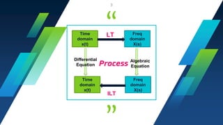
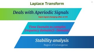
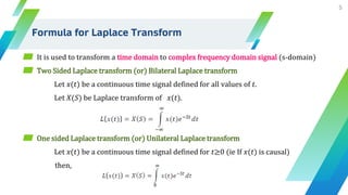
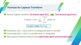
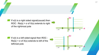
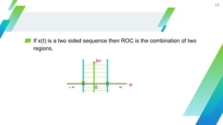
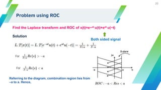
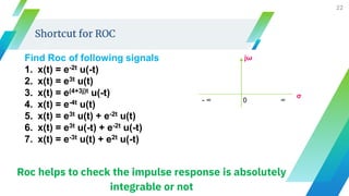
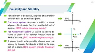
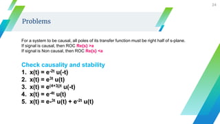
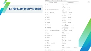
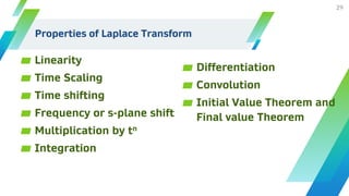
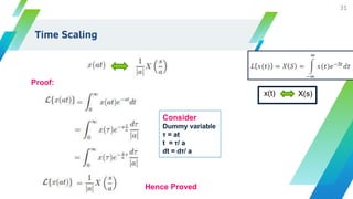
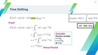
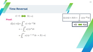
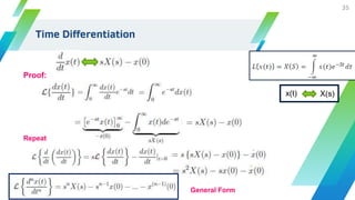
The document discusses the Laplace transform and its properties. It begins by introducing Laplace transform as a tool to transform signals from the time domain to the complex frequency (s-domain). It then provides the Laplace transforms of some elementary signals like impulse, step, ramp functions. It discusses properties like linearity, time shifting, frequency shifting. It also covers the region of convergence, causality, stability analysis using poles in the s-plane. The document provides examples of finding the Laplace transform and analyzing signals based on properties like time shifting and frequency shifting. In the end, it summarizes the convolution property and the initial and final value theorems.

1. Hello!
Nimitha N
Assistant Professor/ECE
nimithaece@rmkcet.ac.in
1
Pierre-Simon Laplace
One of the first scientists to suggest
the existence of black holes

2. Laplace
Transform

3. “
”
Process
3
Time
domain
x(t)
Freq
domain
X(s)
Freq
domain
X(s)
Time
domain
x(t)
Differential
Equation
Algebraic
Equation
LT
ILT

4. Deals with Aperiodic Signals
Input signal changing often at t=0
Stability analysis
Region of Convergence
Time Domain to complex
frequency domain(S-Domain)
4
Laplace Transform

5. Formula for Laplace Transform
5
▰ It is used to transform a time domain to complex frequency domain signal (s-domain)
▰ Two Sided Laplace transform (or) Bilateral Laplace transform
Let 𝑥(𝑡) be a continuous time signal defined for all values of 𝑡.
Let 𝑋(𝑆) be Laplace transform of 𝑥(𝑡).
▰ One sided Laplace transform (or) Unilateral Laplace transform
Let 𝑥(𝑡) be a continuous time signal defined for 𝑡≥0 (ie If 𝑥(𝑡) is causal)
then,

6. ▰ Inverse Laplace transform (S-domain signal 𝑋(𝑆) Time domain signal x(t) )
▰ Transform: x(t)  X(s), where t is integrated and s is variable
▰ Conversely X(s)  x(t), t is variable and s is integrated
▰ The Laplace transform helps to scan exponential signal and sinusoidal signal
6
Complex variable, S= α + jω
Formula for Laplace Transform

7. Laplace transform for elementary signals
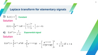
1)
Solution
2)
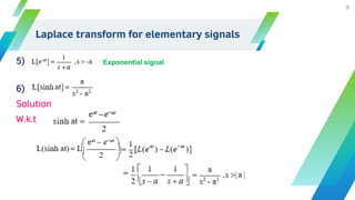
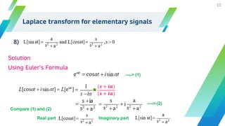
Solution
7
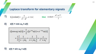
Impulse signal
L[δ(t)]
Step signal
L[u(t)]

8. Laplace transform for elementary signals
3)
Solution
4)
Solution
8
Constant
Exponential signal

9. Laplace transform for elementary signals
5)
6)
Solution
W.k.t
9
Exponential signal

10. Laplace transform for elementary signals
7)
8)
9)
10
Hint
x(t) = cos ω0 t u(t)
x(t) = sin ω0 t u(t)

11. Laplace transform for elementary signals
8)
Solution
Using Euler’s Formula
11
----> (1)
(𝒔 + 𝒊𝒂)
(𝒔 + 𝒊𝒂)
----> (2)
Compare (1) and (2)
Real part Imaginary part

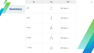
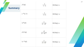
12. Summary
Impulse
Step
12
L[δ(t)] 1
L[u(t)]
1/s
a= ω0
L[1]

13. Advantages of Laplace Transform
▰ Signal which are not convergent on Fourier
transform, will converge in Laplace transform
13

14. Complex S Plane
▰ The most general form of Laplace
transform is
▰ L[x(t)]= X(s) =
𝑵(𝑺)
𝑫(𝑺)
14
LHS RHS
- ∞ 0 ∞
jω
σ
Complex variable, S= α + jω
The zeros are found by setting the numerator polynomial to Zero
The Poles are found by setting the Denominator polynomial to Zero

15. Region of Convergence
The range variation of complex variable ‘s’ (σ) for which the Laplace transform
converges(Finite) is called region of convergence.
Properties of ROC of Laplace Transform
 ROC contains strip lines parallel to jω axis in s-plane.
 ROC doesn’t contain any poles
 If x(t) is absolutely integral and it is of finite duration, then ROC is entire s-
plane.
 If x(t) is a right sided signal(causal) then ROC : Re{s} > σ of X(s) extends
to right of the rightmost pole
 If x(t) is a left sided signal then ROC : Re{s} < σ of X(s) extends to left of
the leftmost pole
 If x(t) is a two sided sequence then ROC is the combination of two regions.
15

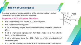
16. Properties of ROC of Laplace Transform
▰ ROC doesn’t contain any poles
▰ If x(t) is absolutely integral and it is of finite duration, then ROC is entire
s-plane.
16
L[e-2t u(t)] 1/(s+2)
1/(-2+2)
Poles, S=-2 = 1/0 = ∞
-a a
x(t)
ROC includes
imaginary axis jω
- ∞ 0 ∞
jω
σ
Impulse signal have ROC is entire S plane

17. ▰ If x(t) is a right sided signal(causal) then
ROC : Re{s} > σ of X(s) extends to right
of the rightmost pole
▰ If x(t) is a left sided signal then ROC :
Re{s} < σ of X(s) extends to left of the
leftmost pole
17
- ∞ 0 ∞
jω
σ
- ∞ 0 ∞
jω
σ

18. ▰ If x(t) is a two sided sequence then ROC is the combination of two
regions.
18
- ∞ 0 ∞
jω
σ

19. Problem using ROC
19
1. Find the Laplace transform and ROC of x(t)=e-at u(t)
Solution
2. Find the Laplace transform and ROC of x(t)=eat u(−t)
Solution
Right sided
signal
Left sided
signal

20. 20
Find the Laplace transform and ROC of x(t)=e−at u(t)+eat u(−t)
Solution
Problem using ROC
Both sided signal
Referring to the diagram, combination region lies from
–a to a. Hence,

21. Shortcut for ROC
▰ Step 1: Compare real part of S complex variable (σ) with real part of
coefficient of power of e
▰ Step 2: Check if the signal is left sided or right sided, then decide < or >
21
Consider L[e-2t u(t)]
Step 1 : σ = -2
Step 2 : σ > -2
ROC is

22. Roc helps to check the impulse response is absolutely
integrable or not
22
Shortcut for ROC
Find Roc of following signals
1. x(t) = e-2t u(-t)
2. x(t) = e3t u(t)
3. x(t) = e(4+3j)t u(-t)
4. x(t) = e-4t u(t)
5. x(t) = e3t u(t) + e-2t u(t)
6. x(t) = e3t u(-t) + e-2t u(-t)
7. x(t) = e-3t u(t) + e2t u(-t)
- ∞ 0 ∞
jω
σ

23. Causality and Stability
▰ For a system to be causal, all poles of its transfer
function must be left half of s-plane.
▰ For causal system: A system is said to be stable
all poles of its transfer function must be left half of
s-plane, (ROC include Imaginary axis jω)
▰ For Anticausal system: A system is said to be
stable all poles of its transfer function must be
RHS of s-plane, (ROC include Imaginary axis jω)
▰ A system is said to be unstable when at least one
pole of its transfer function is shifted to the right
half of s-plane.(ROC doesn’t include Imaginary
axis jω)
23
σ
σ
σ
jω
Poles

24. 24
Problems
Check causality and stability
1. x(t) = e-2t u(-t)
2. x(t) = e3t u(t)
3. x(t) = e(4+3j)t u(-t)
4. x(t) = e-4t u(t)
5. x(t) = e-3t u(t) + e-2t u(t)
For a system to be causal, all poles of its transfer function must be right half of s-plane.
If signal is causal, then ROC Re{s} >a
If signal is Non causal, then ROC Re{s} <a

25. Causality and Stability
25
5. Find the LT and ROC of x(t)=e−3t u(t)+e-2t u(t), Check causality and stability
Solution:
L[x(t)= L[e−3t u(t)+e-2t u(t)]
X(s) =
1
(𝑠+3)
+
1
(𝑠+2)
ROC: Re{s} =σ >-3, Re{s} =σ >-2
ROC: Re{s} =σ >-2
- ∞ -3 -2 0 ∞
jω
σ
Both will converged if Re{s} =σ >-2
Causal and stable

26. Summary
26

27. 27
Summary

28. LT for Elementary signals
28

29. Properties of Laplace Transform
▰ Linearity
▰ Time Scaling
▰ Time shifting
▰ Frequency or s-plane shift
▰ Multiplication by tn
▰ Integration
29
▰ Differentiation
▰ Convolution
▰ Initial Value Theorem and
Final value Theorem

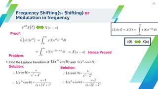
30. Linearity
30
Proof:
x(t) X(s)
Problem Hence Proved
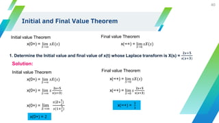
1. Find the Laplace transform of x(t) = 2δ(t)+ 3 u(t)
L[δ(t)] 1
L[u(t)] 1/s
L[x(t)] = L[2δ(t)+ 3 u(t)] = X(s) = 2 L[δ(t)] + 3 L[u(t)]
X(s) = 2+ 3(1/s)
y(t) Y(s)

31. Time Scaling
31
Proof:
x(t) X(s)
Consider
Dummy variable
τ = at
t = τ/ a
dt = dτ/ a
Hence Proved

32. Time Shifting
32
Proof:
x(t) X(s)
Consider
Dummy variable
τ = t-t0
t = τ + t0
dt = dτ
Hence Proved

33. Problem : Time shifting
1. Using Time shifting property, solve
33
Solution: x(t) X(s)
L[u(t-3)] =
𝑒−3𝑠
𝑠
L[u(t-3)]
Using Time shifting property
Given : t0 =3
L[u(t-3)] = X(s) = −∞
∞
𝑢(𝑡 − 3)𝑒−𝑠𝑡
𝑑𝑡
= 3
∞
𝑒−𝑠𝑡
𝑑𝑡
=
𝑒−𝑠𝑡
−𝑠
∞
3
L[u(t-3)] = X(s) = 0
∞
𝑢(𝑡 − 3)𝑒−𝑠𝑡
𝑑𝑡
=
1
−𝑠
𝑒−∞
− 𝑒−3𝑠
𝑒−∞
= 0
L[u(t-3)] =
𝑒−3𝑠
𝑠
L[u(t)] =
1
𝑠
Wkt

34. Time Reversal
34
Proof:
X(s)
x(t)

35. Time Differentiation
35
Proof:
X(s)
x(t)
General Form
Repeat

36. Frequency Shifting(s- Shifting) or
Modulation in frequency
36
Proof:
Hence Proved
x(t) X(s)
Problem:
Solution:
1. Find the Laplace transform of and
Solution:

37. 2. solve
37
Solution:
= e-6 L[e-3(t-2) u(t-2)]
Given : t0 =2
= e-6 L[e-3t] e-2s
Wkt, L[e-at ] = (1/s+a)
= e-2s e-6(1/s+3)
=
e−(2s+6)
(s+3)
=
e−2(s+3)
(s+3)
x(t) X(s)
= L[e-3(t-2+2) u(t-2)]
L[u(t-2)] =
𝑒−2𝑠
𝑠
Sub : s by s+3
=
𝑒−2(𝑠+3)
(𝑠+3)
Problem : Frequency Shifting+ Time Shifting

38. Frequency Differentiation
38
X(s)
x(t)
1.Determine LT of
Solution:
n=1
L[t u(t)] = (-1)
𝑑
𝑑𝑠
L[u(t)]
Wkt
L[u(t)] = 1/s
= (-1)
𝑑
𝑑𝑠
(
1
𝑠
)
= (-1)
𝑑
𝑑𝑠
( 𝑠−1
)
= (-1) ( −𝑠−2
)
= 1/𝑠2
L[t u(t)]
L[t2 u(t)]= 2/𝑠3
Similarly
Ramp signal
Parabolic signal

39. Convolution Theorem
39
L[x1(t) * x2(t)] X1(s) . X2(s)
1.Consider x1(t) = u(t) and x2(t) =𝑒−5𝑡
u(t)
Y(s) = X1(s) . X2(s)
L[x1(t)] =
1
𝑠
L[x2(t)] =
1
𝑠+5
Y(s) =
𝐴
𝑠
+
𝐵
𝑠+5
Y(s) =
1
𝑠
.
1
𝑠+5
=
𝐴 𝑠+5 +𝐵𝑠
𝑠(𝑆+5)
Y(s) =
1
𝑠(𝑠+5)
Sub s=0
A= 1/5
Sub s=-5
B= -1/5
Y(s) =
1/5
𝑠
+
−1/5
𝑠+5
Sub A and B in (1)
(1)
ILT [Y(s)] = y(t)
y(t) =
1
5
u(t) -
1
5
𝑒−5𝑡
u(t)

40. Initial and Final Value Theorem
40
Initial value Theorem Final value Theorem
x(∞+) = lim
𝑆→0
𝑠𝑋(𝑠)
x(0+) = lim
𝑆→∞
𝑠𝑋(𝑠)
1. Determine the Initial value and final value of x(t) whose Laplace transform is X(s) =
𝟐𝒔+𝟓
𝒔(𝒔+𝟑)
x(0+) = lim
𝑆→∞
𝑠𝑋(𝑠)
Initial value Theorem
Solution:
x(0+) = lim
𝑆→∞
𝑠
𝟐𝒔+𝟓
𝒔(𝒔+𝟑)
x(0+) = lim
𝑆→∞
𝑠(𝟐+
5
𝑠
)
𝑠(1+
3
𝑠
)
x(0+) = 2
Final value Theorem
x(∞+) = lim
𝑆→0
𝑠𝑋(𝑠)
x(∞+) = lim
𝑆→0
𝑠
𝟐𝒔+𝟓
𝒔(𝒔+𝟑)
x(∞+) =
5
3

41. Initial and Final Value Theorem
41
Initial value Theorem Final value Theorem
x(∞+) = lim
𝑆→0
𝑠𝑋(𝑠)
x(0+) = lim
𝑆→∞
𝑠𝑋(𝑠)
2. Determine the Initial value and final value of x(t) whose Laplace transform is X(s) =
𝒔+𝟓
(𝒔𝟐+𝟑𝒔+𝟐)
x(0+) = lim
𝑆→∞
𝑠𝑋(𝑠)
Initial value Theorem
Solution:
x(0+) = 1
Final value Theorem
x(∞+) = lim
𝑆→0
𝑠𝑋(𝑠)
x(∞+) = 0
x(0+) = lim
𝑆→∞
𝑠
𝒔+𝟓
(𝒔𝟐+𝟑𝒔+𝟐)
x(0+) = lim
𝑆→∞
𝑠
𝒔(𝟏+
𝟓
𝒔
)
𝒔𝟐(𝟏+
𝟑
𝒔
+
𝟐
𝒔𝟐)
x(∞+) = lim
𝑆→0
𝑠
𝒔+𝟓
(𝒔𝟐+𝟑𝒔+𝟐)

42. Inverse Laplace transform using Partial
fraction
42
Partial fraction
types
01
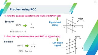
L[eat]u(t) = Roc, Re{s} σ > a
L[-e-at]u(-t) = Roc, Re{s} σ < a
02
03

43. Problems ( Simple Poles)
43
1.Determine Inverse LT of
Solution:
𝐴 𝑠 + 1 𝑠 + 2 + 𝐵𝑠 𝑠 + 2 + 𝐶𝑠(𝑠 + 1)
𝑠(𝑠 + 1)(𝑠 + 2)
2 = 𝐴 𝑠 + 1 𝑠 + 2 + 𝐵𝑠 𝑠 + 2 + 𝐶𝑠(𝑠 + 1)
Sub S= 0
2 = 𝐴 1 2
A = 1
Sub S= -1
2 = 𝐴 −1 + 1 −1 + 2 + 𝐵(−1) −1 + 2 + 𝐶(−1)(−1 + 1)
B = -2
(1)

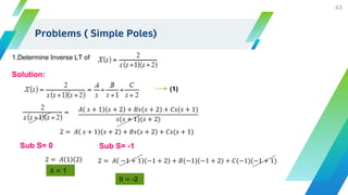
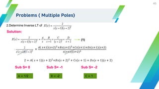
44. 44
Sub S= -2
2 = 𝐴 −2 + 1 −2 + 2 + 𝐵(−2) −2 + 2 + 𝐶(−2)(−2 + 1)
C = 1
Sub A, B and C in (1)
X(s) =
𝐴
𝑠
+
𝐵
(𝑠 + 1)
+
𝐶
(𝑠 + 2)
X(s) =
1
𝑠
+
−2
(𝑠 + 1)
+
1
(𝑠 + 2)
ILT [X(s)] = x(t)
x(t) =𝑢 𝑡 − 2 𝑒−𝑡
𝑢 𝑡 + 𝑒−2𝑡
𝑢(𝑡)
𝑒−𝑎𝑡
𝑢 𝑡 =
1
(𝑠 + 𝑎)

45. 45
Problems ( Multiple Poles)
2.Determine Inverse LT of
Solution:
=
𝐴 𝑠+1 (𝑠+2)2+𝐵𝑠(𝑠+2)2+𝐶𝑠 𝑠+1 +𝐷𝑠(𝑠+1)(𝑠+2)
𝑠(𝑠+1)(𝑠+2)2
2 = 𝐴 𝑠 + 1 (𝑠 + 2)2
+𝐵𝑠(𝑠 + 2)2
+ 𝐶𝑠 𝑠 + 1 + 𝐷𝑠(𝑠 + 1)(𝑠 + 2)
C = 1
Sub S= 0
A = 1/2
Sub S= -1
B = -2
Sub S= -2
(1)

46. 46
2 = 𝐴 𝑠 + 1 (𝑠 + 2)2
+𝐵𝑠(𝑠 + 2)2
+ 𝐶𝑠 𝑠 + 1 + 𝐷𝑠(𝑠 + 1)(𝑠 + 2)
2 = 𝐴 𝑠 + 1 (𝑠2
+ 2𝑠 + 4) + 𝐵𝑠(𝑠2
+ 2𝑠 + 4) + 𝐶𝑠 𝑠 + 1 + 𝐷𝑠(𝑠2
+ 3𝑠 + 2)
2 = 𝐴𝑠3
+ 2𝐴𝑠2
+ 4𝐴𝑠 + 𝐴𝑠2
+ 2𝐴𝑠 + 4𝐴 + 𝐵𝑠3
+ 2𝐵𝑠2
+ 4𝐵𝑠 + 𝐶𝑠2
+ 𝐶𝑠 + 𝐷𝑠3
+ 3𝐷𝑠2
+ 2𝐷𝑠)
Equating 𝑡ℎ𝑒 𝑐𝑜𝑒𝑓𝑓𝑖𝑐𝑒𝑛𝑡 𝑜𝑓 𝑠3
0= A+B+D
0= 0.5-2+D D= 1.5 or 3/2
X(s) =
𝐴
𝑠
+
𝐵
(𝑠+1)
+
𝐶
(𝑠+2)2 +
𝐷
𝑠+2
Sub A,B,C and D in (1)
X(s) =
0.5
𝑠
−
2
(𝑠+1)
+
1
(𝑠+2)2 +
1.5
𝑠+2
x(t) =0.5𝑢 𝑡 − 2 𝑒−𝑡
𝑢 𝑡 + 𝑡𝑒−2𝑡
𝑢 𝑡 + 1.5 𝑒−2𝑡
𝑢 𝑡
ILT [X(s)] = x(t)

47. 47
Problems ( Complex Poles)
3.Determine Inverse LT of X(s) =
(2𝑠+1)
(𝑠+1)(𝑠2+2𝑠+2)
Solution:
X(s) =
(2𝑠+1)
(𝑠+1)(𝑠2+2𝑠+2)
X(s) =
𝐴
(𝑠+1)
+
𝐵𝑠+ 𝐶
(𝑠2+2𝑠+2)
(2𝑠 + 1)
(𝑠 + 1)(𝑠2 + 2𝑠 + 2)
=
𝐴
(𝑠 + 1)
+
𝐵𝑠 + 𝐶
(𝑠2 + 2𝑠 + 2)
(2𝑠 + 1)
(𝑠 + 1)(𝑠2 + 2𝑠 + 2)
=
𝐴 𝑠2
+ 2𝑠 + 2 + 𝐵𝑠 + 𝐶(𝑠 + 1)
(𝑠 + 1)(𝑠2 + 2𝑠 + 2)
C = 3 A = -1
Equating 𝑡ℎ𝑒 𝑐𝑜𝑒𝑓𝑓𝑖𝑐𝑒𝑛𝑡 𝑜𝑓 𝑠2
, s and constant
B = 1
(1)

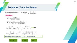
48. 48
X(s) =
𝐴
(𝑠 + 1)
+
𝐵𝑠 + 𝐶
(𝑠2 + 2𝑠 + 2)
(1)
Sub A,B and C in (2)
X(s) =
𝐴
(𝑠 + 1)
+
𝐵𝑠 + 𝐶
(𝑠 + 1)2 + 1)
(2)
X(s) =
−1
(𝑠 + 1)
+
𝑠 + 3
(𝑠 + 1)2 + 1)
X(s) =
−1
(𝑠 + 1)
+
𝑠 + 1 + 2
(𝑠 + 1)2 + 1
X(s) =
−1
(𝑠+1)
+
𝑠+1
(𝑠+1)2+1
+
2
(𝑠+1)2+1
ILT [X(s)] = x(t) x(t) =𝑒−𝑡
𝑢 𝑡 − 𝑒−𝑡
cos 𝑡 𝑢 𝑡 + 2𝑒−𝑡
sin 𝑡 𝑢 𝑡
L[𝑒−𝑎𝑡
cos t] 𝑠 + 𝑎
(𝑠 + 𝑎)2 + 𝑎2
L[𝑒−𝑎𝑡
sin t]
𝑎
(𝑠 + 𝑎)2 + 𝑎2
Problems ( Complex Poles)

49. Problem Using RoC
49
4.Determine Inverse LT of X(s) =
4
(𝑠+2)(𝑠+4)
if ROC (i) -2 >Re(s) > -4 , (ii) Re(s) < -4
=
𝐴 𝑠+4 +𝐵 𝑠+2
(𝑠+2)(𝑠+4)
X(s) =
4
(𝑠+2)(𝑠+4)
=
𝐴
(𝑠+2)
+
𝐵
(𝑠+4)
4
(𝑠+2)(𝑠+4)
A = 2 B = −2
X(s) =
2
(𝑠+2)
-
2
(𝑠+4)
Sub in (1)
(1)
x(t) =2𝑒−2𝑡
𝑢 𝑡 − 2𝑒−4𝑡
𝑢 𝑡

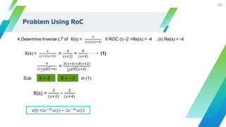
50. 50
(i) ROC -2 >Re(s) > -4
(ii) ROC Re(s) < -4
x(t) = −2𝑒−2𝑡
𝑢 −𝑡 − 2𝑒−4𝑡
𝑢 𝑡
x(t) =2𝑒−2𝑡
𝑢 𝑡 − 2𝑒−4𝑡
𝑢 𝑡
- ∞ 0 ∞
jω
σ
Re(s)<-2 and Re(s)> -4
L[eat]u(t) = Roc, Re{s} σ > a
L[-e-at]u(-t) = Roc, Re{s} σ < a
x(t) =2𝑒−2𝑡
𝑢 𝑡 − 2𝑒−4𝑡
𝑢 𝑡
- ∞ 0 ∞
jω
σ
x(t) = −2𝑒−2𝑡
𝑢 −𝑡 + 2𝑒−4𝑡
𝑢 −𝑡
Problem Using RoC

51. 51
(iii) ROC Re(s) > 2
x(t) =2𝑒−2𝑡
𝑢 𝑡 − 2𝑒−4𝑡
𝑢 𝑡
x(t) =2𝑒−2𝑡
𝑢 𝑡 − 2𝑒−4𝑡
𝑢 𝑡
- ∞ 0 ∞
jω
σ
Problem Using RoC

52. THANK YOU

53. 53
https://www.tutorialspoint.com/signals_and_systems/region_of_c
onvergence.htm
http://jntuhsd.in/uploads/programmes/Module16_LT_14.0_.2017_
.PDF (Properties)