The document discusses various methods for computing the inverse z-transform including inspection, partial fraction expansion, and power series expansion. It provides examples to illustrate each method. The inverse z-transform finds the original time domain sequence from its z-transform. Key properties like linearity, time shifting, and convolution are also covered.

1. The Inverse z-Transform
In science one tries to tell people, in such a way
as to be understood by everyone, something
that no one ever knew before.
But in poetry, it's the exact opposite.
Paul Dirac
Content and Figures are from Discrete-Time Signal Processing, 2e by Oppenheim, Shafer, and Buck, ©1999-2000 Prentice Hall Inc.

2. 351M Digital Signal Processing 2
The Inverse Z-Transform
• Formal inverse z-transform is based on a Cauchy integral
• Less formal ways sufficient most of the time
– Inspection method
– Partial fraction expansion
– Power series expansion
• Inspection Method
– Make use of known z-transform pairs such as
– Example: The inverse z-transform of
[ ] az
az1
1
nua 1
Zn
>
−
 →← −
( ) [ ] [ ]nu
2
1
nx
2
1
z
z
2
1
1
1
zX
n
1






=→>
−
=
−

3. 351M Digital Signal Processing 3
Inverse Z-Transform by Partial Fraction Expansion
• Assume that a given z-transform can be expressed as
• Apply partial fractional expansion
• First term exist only if M>N
– Br is obtained by long division
• Second term represents all first order poles
• Third term represents an order s pole
– There will be a similar term for every high-order pole
• Each term can be inverse transformed by inspection
( )
∑
∑
=
−
=
−
= N
0k
k
k
M
0k
k
k
za
zb
zX
( )
( )∑∑∑ =
−
≠=
−
−
=
−
−
+
−
+=
s
1m
m1
i
m
N
ik,1k
1
k
k
NM
0r
r
r
zd1
C
zd1
A
zBzX

4. 351M Digital Signal Processing 4
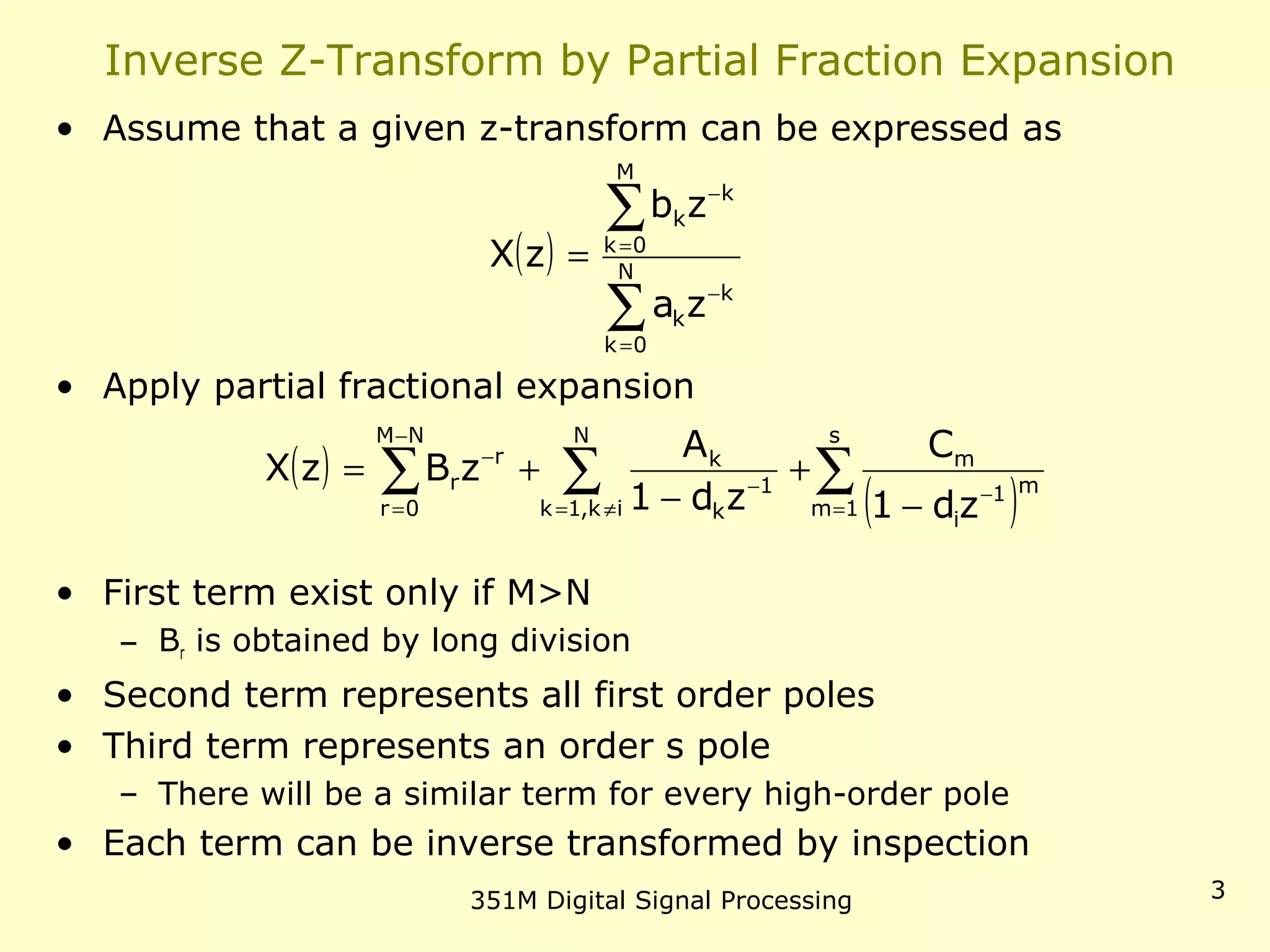
Partial Fractional Expression
• Coefficients are given as
• Easier to understand with examples
( )
( )∑∑∑ =
−
≠=
−
−
=
−
−
+
−
+=
s
1m
m1
i
m
N
ik,1k
1
k
k
NM
0r
r
r
zd1
C
zd1
A
zBzX
( ) ( ) kdz
1
kk zXzd1A =
−
−=
( ) ( )
( ) ( )[ ] 1
idw
1s
ims
ms
ms
i
m wXwd1
dw
d
d!ms
1
C
−
=
−
−
−
−






−
−−
=

5. 351M Digital Signal Processing 5
Example: 2nd
Order Z-Transform
– Order of numerator is smaller than denominator (in terms of z-1
)
– No higher order pole
( )
2
1
z:ROC
z
2
1
1z
4
1
1
1
zX
11
>






−





−
=
−−
( )






−
+






−
=
−− 1
2
1
1
z
2
1
1
A
z
4
1
1
A
zX
( ) 1
4
1
2
1
1
1
zXz
4
1
1A 1
4
1
z
1
1 −=














−
=





−= −
=
−
( ) 2
2
1
4
1
1
1
zXz
2
1
1A 1
2
1
z
1
2 =














−
=





−= −
=
−

6. 351M Digital Signal Processing 6
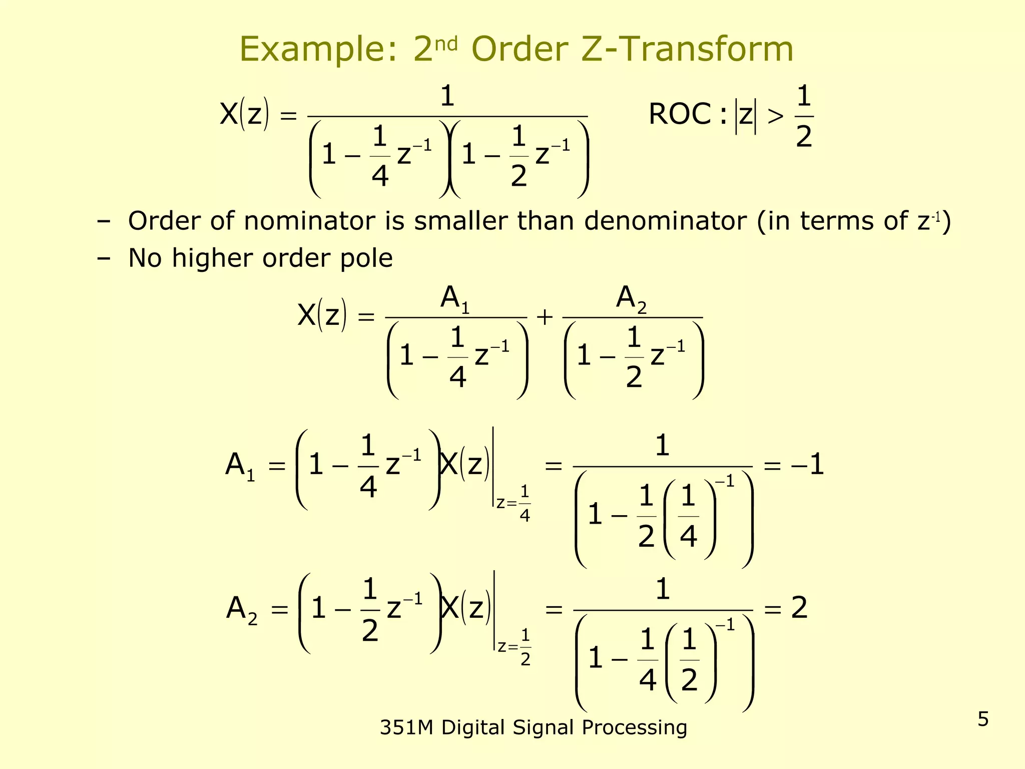
Example Continued
• ROC extends to infinity
– Indicates right sided sequence
( )
2
1
z
z
2
1
1
2
z
4
1
1
1
zX
11
>






−
+






−
−
=
−−
[ ] [ ] [ ]nu
4
1
-nu
2
1
2nx
nn












=

7. 351M Digital Signal Processing 7
Example #2
• Long division to obtain Bo
( ) ( )
( )
1z
z1z
2
1
1
z1
z
2
1
z
2
3
1
zz21
zX
11
21
21
21
>
−





−
+
=
+−
++
=
−−
−
−−
−−
1z5
2z3z
2
1z2z1z
2
3
z
2
1
1
12
1212
−
+−
+++−
−
−−
−−−−
( )
( )11
1
z1z
2
1
1
z51
2zX
−−
−
−





−
+−
+=
( ) 1
2
1
1
z1
A
z
2
1
1
A
2zX −
− −
+
−
+=
( ) 9zXz
2
1
1A
2
1
z
1
1 −=





−=
=
−
( ) ( ) 8zXz1A
1z
1
2 =−=
=
−

8. 351M Digital Signal Processing 8
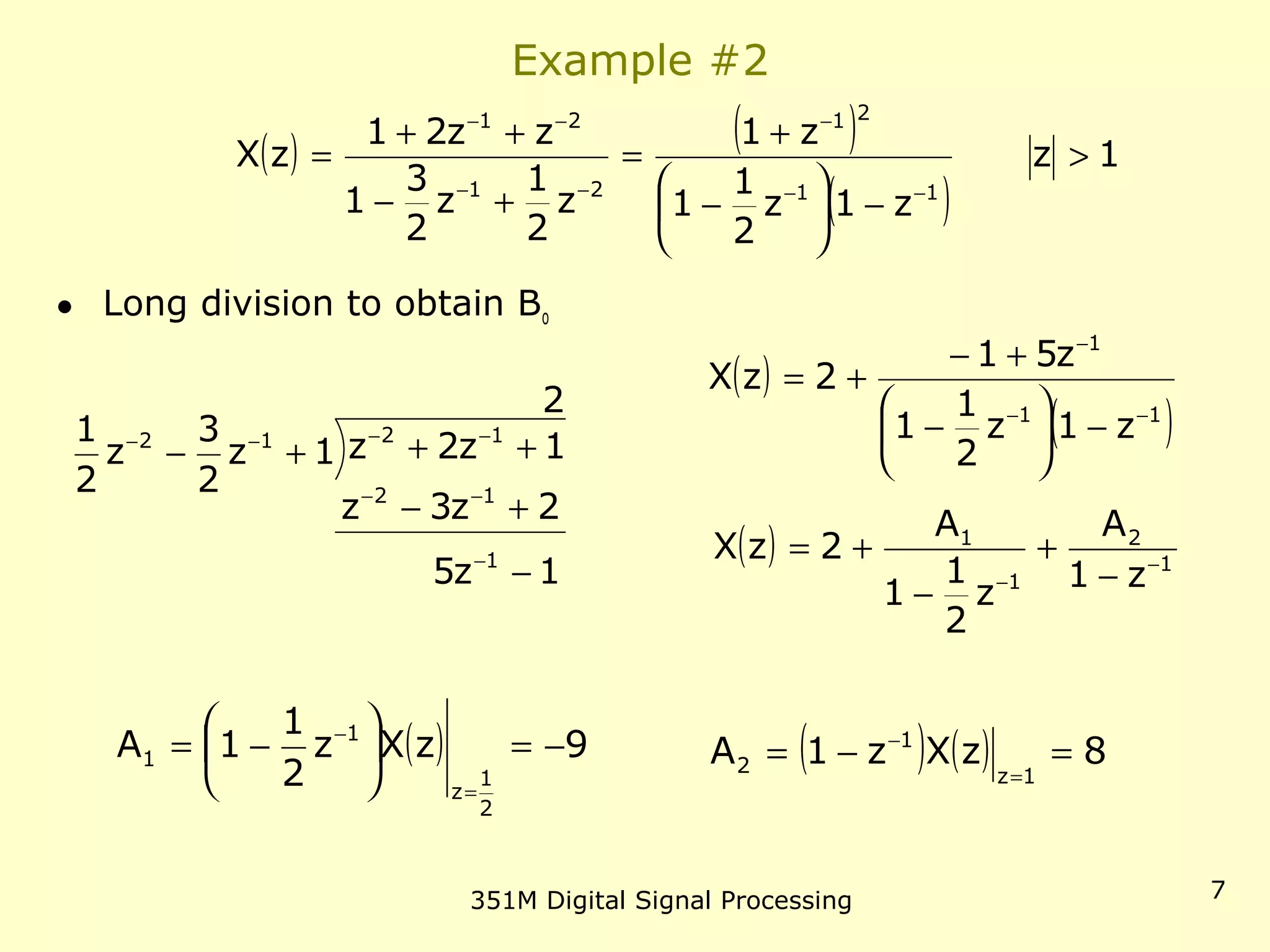
Example #2 Continued
• ROC extends to infinity
– Indicates right-sides sequence
( ) 1z
z1
8
z
2
1
1
9
2zX 1
1
>
−
+
−
−= −
−
[ ] [ ] [ ] [ ]n8u-nu
2
1
9n2nx
n






−δ=

9. 351M Digital Signal Processing 9
Inverse Z-Transform by Power Series Expansion
• The z-transform is power series
• In expanded form
• Z-transforms of this form can generally be inversed easily
• Especially useful for finite-length series
• Example
( ) [ ]∑
∞
−∞=
−
=
n
n
znxzX
( ) [ ] [ ] [ ] [ ] [ ]  ++++−+−+= −− 2112
z2xz1x0xz1xz2xzX
( ) ( )( )
12
1112
z
2
1
1z
2
1
z
z1z1z
2
1
1zzX
−
−−−
+−−=
−+





−=
[ ] [ ] [ ] [ ] [ ]1n
2
1
n1n
2
1
2nnx −δ+δ−+δ−+δ=
[ ]









=
=
=−
−=−
−=
=
2n0
1n
2
1
0n1
1n
2
1
2n1
nx

10. 351M Digital Signal Processing 10
Z-Transform Properties: Linearity
• Notation
• Linearity
– Note that the ROC of combined sequence may be larger than
either ROC
– This would happen if some pole/zero cancellation occurs
– Example:
• Both sequences are right-sided
• Both sequences have a pole z=a
• Both have a ROC defined as |z|>|a|
• In the combined sequence the pole at z=a cancels with a zero at z=a
• The combined ROC is the entire z plane except z=0
• We did make use of this property already, where?
[ ] ( ) x
Z
RROCzXnx = →←
[ ] [ ] ( ) ( ) 21 xx21
Z
21 RRROCzbXzaXnbxnax ∩=+ →←+
[ ] [ ] [ ]N-nua-nuanx nn
=

11. 351M Digital Signal Processing 11
Z-Transform Properties: Time Shifting
• Here no is an integer
– If positive the sequence is shifted right
– If negative the sequence is shifted left
• The ROC can change the new term may
– Add or remove poles at z=0 or z=∞
• Example
[ ] ( ) x
nZ
o RROCzXznnx o
= →←− −
( )
4
1
z
z
4
1
1
1
zzX
1
1
>












−
=
−
−
[ ] [ ]1-nu
4
1
nx
1-n






=

12. 351M Digital Signal Processing 12
Z-Transform Properties: Multiplication by Exponential
• ROC is scaled by |zo|
• All pole/zero locations are scaled
• If zo is a positive real number: z-plane shrinks or expands
• If zo is a complex number with unit magnitude it rotates
• Example: We know the z-transform pair
• Let’s find the z-transform of
[ ] ( ) xoo
Zn
o RzROCz/zXnxz = →←
[ ] 1z:ROC
z-1
1
nu 1-
Z
> →←
[ ] ( ) [ ] ( ) [ ] ( ) [ ]nure
2
1
nure
2
1
nuncosrnx
njnj
o
n oo ω−ω
+=ω=
( ) rz
zre1
2/1
zre1
2/1
zX 1j1j oo
>
−
+
−
= −ω−−ω

13. 351M Digital Signal Processing 13
Z-Transform Properties: Differentiation
• Example: We want the inverse z-transform of
• Let’s differentiate to obtain rational expression
• Making use of z-transform properties and ROC
[ ] ( )
x
Z
RROC
dz
zdX
znnx =− →←
( ) ( ) azaz1logzX 1
>+= −
( ) ( )
1
1
1
2
az1
1
az
dz
zdX
z
az1
az
dz
zdX
−
−
−
−
+
=−⇒
+
−
=
[ ] ( ) [ ]1nuaannx
1n
−−=
−
[ ] ( ) [ ]1nu
n
a
1nx
n
1n
−−=
−

14. 351M Digital Signal Processing 14
Z-Transform Properties: Conjugation
• Example
[ ] ( ) x
**Z*
RROCzXnx = →←
( ) [ ]
( ) [ ] [ ]
( ) [ ] ( ) [ ] [ ]{ }nxZznxznxzX
znxznxzX
znxzX
n
n
n
n
n
n
n
n
n
n
∗
∞
−∞=
−∗
∞
−∞=
∗∗∗∗
∞
−∞=
∗
∗
∞
−∞=
−∗
∞
−∞=
−
===
=





=
=
∑∑
∑∑
∑

15. 351M Digital Signal Processing 15
Z-Transform Properties: Time Reversal
• ROC is inverted
• Example:
• Time reversed version of
[ ] ( )
x
Z
R
1
ROCz/1Xnx = →←−
[ ] [ ]nuanx n
−= −
[ ]nuan
( ) 1
11-
1-1
az
za-1
za-
az1
1
zX −
−
−
<=
−
=

16. 351M Digital Signal Processing 16
Z-Transform Properties: Convolution
• Convolution in time domain is multiplication in z-domain
• Example:Let’s calculate the convolution of
• Multiplications of z-transforms is
• ROC: if |a|<1 ROC is |z|>1 if |a|>1 ROC is |z|>|a|
• Partial fractional expansion of Y(z)
[ ] [ ] ( ) ( ) 2x1x21
Z
21 RR:ROCzXzXnxnx ∩ →←∗
[ ] [ ] [ ] [ ]nunxandnuanx 2
n
1 ==
( ) az:ROC
az1
1
zX 11 >
−
= −
( ) 1z:ROC
z1
1
zX 12 >
−
= −
( ) ( ) ( )
( )( )1121
z1az1
1
zXzXzY −−
−−
==
( ) 1z:ROCasume
az1
1
z1
1
a1
1
zY 11
>





−
−
−−
= −−
[ ] [ ] [ ]( )nuanu
a1
1
ny 1n+
−
−
=