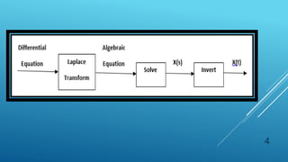
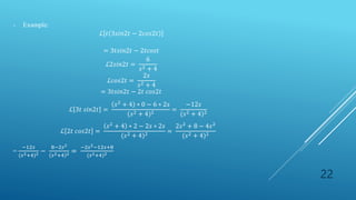
This document discusses the Laplace transform, which is used to analyze linear systems. It provides examples of common Laplace transforms, such as the unit step function, exponential functions, and trigonometric functions. Properties of the Laplace transform are also covered, including: multiplication by a constant, linearity, multiplication by an exponential, and multiplication by time (frequency derivative). The document aims to introduce engineering students to the Laplace transform and its applications in differential equations.

1. MINISTRY OF SCIENTIFIC EDUCATION AND HIGHER RESEARCHES
NORTHERN TECHNICAL UNIVERSITY
ENGINEERING TECHNICAL COLLEGE / MOSUL
DEPARTMENT OF COMPUTER TECHNOLOGY
1
ENGINEERING ANALYSIS LECTURE
DEPARTMENT OF COMPUTER
TECHNOLOGY –THIRD CLASS
2018 -2019
ARJUWAN MOHAMMED ABDULJAWAD
ALJAWADI
LECTURER

2. 2
- ENGINEERING ANALYSIS
One of important transforms used in linear- system analysis. It is
named in honor of the great French mathematician, Pierre Simon De
Laplace (1749-1827).

3. 3
- Purpose of Laplace Transform
• To convert from one type of operation to another
operations of different types in more simple form.
• A well-known technique for solving differential
equations.

4. 4

5. - THE TIME DOMAIN SIGNAL IS CONTINUOUS , EXTENDS
TO:
1. POSITIVE AND NEGATIVE INFINITY.
2. PERIODIC OR APERIODIC SIGNAL
5
- Laplace Transform Definition:
The Laplace transform F(s) of a time function F (t) is given by the
integral:

6. 6
This definition is called the bilateral, or two-sided, Laplace transform—hence, the
subscript b. Notice that the bilateral Laplace transform integral becomes the Fourier
transform integral if is replaced by (𝑗𝑤 ) . The Laplace transform variable is
complex 𝑠 = 𝛼 + 𝑗𝑤, we can rewrite (1) as:
𝐹 𝑠 =
−∞
∞
𝑓(𝑡)𝑒−(𝜎+𝑗𝜔)𝑡
𝑑𝑡
=
−∞
∞
𝑓(𝑡)𝑒−𝜎𝑡
𝑒−𝑗𝑤
𝑑𝑡

7. 7
𝑓 𝑡 𝑖𝑠 𝑧𝑒𝑟𝑜 𝑓𝑜𝑟 𝑎𝑙𝑙 𝑡 < 0 Thus the first integral in above equation
is zero.
The resulting transform, called the unilateral, or single-sided Laplace
transform, is given by:

8. 8
THE LAPLACE-TRANSFORM VARIABLE S IS COMPLEX, AND WE
DENOTE ITS REAL PART AS ∝ AND ITS IMAGINARY PART AS
𝑗𝑤 THAT IS: 𝑠 = ∝ +𝑗𝑤
The S-plane

9. 9
Some Elementary Functions F(t) and their Laplace Transform
F(t) F(s)
U(t) 1
s
t 1/s2
tn n!/ sn+1
e−at
1
s + a
eat
1
s − a
sin wt w/s2+w2
cos at s/s2+a2
sin hat w/s2- w2
cos hat s/s2- w2

10. 10
- Laplace Transform of some important functions
1. Laplace Transform of a unit –step function 𝑓(𝑡) = 1.

11. 11
2. Laplace Transform of 𝑓(𝑡) = 𝑒𝑎𝑡

12. 12
3. Laplace Transform of 𝑓(𝑡) = 𝑡𝑛
Where n= (1,2,3,4,…………………………….)
f s = 0
∞
e−st tn .dt
udv = uv − v . du
U=tn , du = (𝑛 𝑡𝑛−1) , dv= e−st , v=-
e−st
s
f s = − e−st.tn/s |- 0
∞
𝑛
𝑒−𝑠𝑡
𝑠
.tn-1.dt

13. 13
The first term limits will be form (0 to ∞) by substituting it yields zero while the second
term by substitution we get:
f s = 0
∞ −ne−st
s
n tn-1.dt
u=ntn-1 , du=n(n-1)tn-2 , dv=
e−st
s
, v= - e−st/s2
f s = ne−st
tn-1 /s2 | - 0
∞
−n(n − 1)tn-2/s2 .e−st
. dt
f s = 0
∞
n(n − 1)e−st tn-2 /s2 .dt
Then after n times integration we have :
f s =
0
∞
n!
sn
tn−ne−st. dt
f s =
0
∞
n!
sn
e−st. dt
=
n!
sn+1 e−st
| =
n!
sn+1

14. NOTE: IN THIS SAME METHOD YOU CAN FIND LAPLACE TRANSFORM OF COS 𝑤𝑡
14
𝐿𝑎𝑝𝑙𝑎𝑐𝑒 [𝑠𝑖𝑛 𝑤𝑡] =
0
∞
𝑠𝑖𝑛𝑤𝑡𝑒−𝑠𝑡
. 𝑑𝑡
𝑒𝑗𝑤𝑡
= 𝑐𝑜𝑠 𝑤𝑡 + 𝑗𝑠𝑖𝑛 𝑤𝑡
𝑠𝑖𝑛 𝑤𝑡 𝑖𝑠 𝑡ℎ𝑒 𝐼𝑚𝑎𝑔𝑖𝑛𝑎𝑟𝑦 𝑝𝑎𝑟𝑡 (𝐼𝑚) 𝑜𝑓 𝑒𝑗𝑤𝑡
𝑠𝑖𝑛 𝑤𝑡 = 𝐼𝑚 (𝑒𝑗𝑤𝑡
)
𝐿𝑎𝑝𝑙𝑎𝑐𝑒 [𝑠𝑖𝑛 𝑤𝑡] = 𝐼𝑚
0
∞
𝑒𝑗𝑤𝑡𝑒−𝑠𝑡. 𝑑𝑡
= 𝐼𝑚
0
∞
𝑒−(𝑠−𝑗𝑤). 𝑑𝑡
= 𝐼𝑚 [−
𝑒− 𝑠−𝑗𝑤 𝑡
(𝑠 − 𝑗𝑤)
] = 𝐼𝑚 [0 − (−
𝑒0
𝑠 − 𝑗𝑤)
)
= 𝐼𝑚
1
𝑠 − 𝑗𝑤
= 𝐼𝑚 [
1
𝑎 − 𝑗𝑤
∗
𝑠 + 𝑗𝑤
𝑠 + 𝑗𝑤
]
= 𝐼𝑚 (𝑠 + 𝑗𝑤) / (𝑠2 + 𝑤2) = 𝑤 / (𝑠2 + 𝑤2)
4. Laplace Transform of f t = 𝑠𝑖𝑛 𝑤𝑡

15. 5. LAPLACE TRANSFORM OF F T = 𝐶𝑜𝑠ℎ(𝑎𝑡)
15
𝐶𝑜𝑠ℎ(𝑎𝑡) =
𝑒𝑎𝑡
+ 𝑒−𝑎𝑡
2
ℒ cosh 𝑎𝑡 =
1
2
1
𝑠 − 𝑎
+
1
𝑠 + 𝑎
=
1
2
∗ [
𝑠 + 𝑎 + 𝑠 − 𝑎
(𝑠 − 𝑎)(𝑠 + 𝑎)
]
=
1
2
∗ [
2𝑠
𝑠2 + 𝑎𝑠 − 𝑎𝑠 − 𝑎2
]
=
1
2
[
2𝑠
𝑠2 − 𝑎2
]
=
𝑠
𝑠2 − 𝑎2

16. 16
- Laplace Transform Properties:
1. Multiplication by Constant:
ℒ 𝑘. 𝐹 𝑡 = 0
∞
𝑘. 𝐹 𝑡 𝑒−𝑠𝑡
. 𝑑𝑡
= k. 0
∞
𝐹(𝑡)𝑒−𝑠𝑡 . 𝑑𝑡
=𝑘. 𝐹(𝑠)
Example:
ℒ3. 𝑒2𝑡
= 3.
1
𝑠 − 2
=
3
𝑠 − 2

17. 17
2. Linearity:
If 𝐹 𝑡 = 𝐹1 𝑡 + 𝐹2 𝑡
ℒ 𝐹 𝑡 = 0
∞
𝐹(𝑡)𝑒−𝑠𝑡
.dt
= 0
∞
𝐹1 𝑡 + 𝐹2 𝑡 𝑒−𝑠𝑡
. 𝑑𝑡
= 0
∞
𝐹1 𝑡 𝑒−𝑠𝑡. 𝑑𝑡 + 0
∞
𝐹2 𝑡 𝑒−𝑠𝑡. 𝑑𝑡
= ℒ 𝐹1 𝑡 + ℒ[𝐹2 𝑡 ] = 𝐹1 𝑠 + 𝐹2(𝑠)
If 𝐹 𝑡 = 𝑎1𝐹1 𝑡 + 𝑎2𝐹2 𝑡
Where a1 and a2 are constants
Then ℒ[𝑎1𝐹1 𝑡 + 𝑎2𝐹2 𝑡 ]
= 𝑎1ℒ 𝐹1 𝑡 + 𝑎2ℒ 𝐹2 𝑡

18. 18
Examples:
1. ℒ[2𝑠𝑖𝑛3𝑡 + 𝑐𝑜𝑠3𝑡]
= 2 ℒ 𝑠𝑖𝑛3𝑡 + ℒ[𝑐𝑜𝑠3𝑡]
= 2.
3
𝑠2+9
+
𝑠
𝑠2+9
=
𝑠+6
𝑠2+9
2. ℒ[ 4 𝑒5𝑡
+ 6𝑡3
− 3𝑠𝑖𝑛4𝑡 + 2𝑐𝑜𝑠2𝑡]
=
4
𝑠 − 5
+
6.3!
𝑠4
−
12
𝑠2 + 16
+
2𝑠
𝑠2 + 4
=
4
𝑠 − 5
+
36
𝑠4 −
12
𝑠2 + 16
+
2𝑠
𝑠2 + 4
- Home Work:
- ℒ[3𝑐𝑜𝑠6𝑡 − 5𝑠𝑖𝑛6]
- ℒ[3𝑡10
− 8𝑒−3𝑡
+ 5𝑐𝑜𝑠3𝑡 + 4𝑠𝑖𝑛2𝑡]
- ℒ[3𝑐𝑜𝑠5𝑡 − 4𝑠𝑖𝑛ℎ5𝑡]

19. 19
3. Multiplication by exponential:
𝑓1 𝑡 = 𝑓 𝑡 𝑒−𝑎𝑡
ℒ 𝑓 𝑡 𝑒−𝑎𝑡
=
0
∞
𝑓 𝑡 𝑒−𝑎𝑡
𝑒−𝑠𝑡
0
∞
𝑓 𝑡 𝑒− 𝑠+𝑎 𝑡
. 𝑑𝑡 Then 𝑓(𝑠 + 𝑎)
The transform ℒ 𝑓 𝑡 𝑒−𝑎𝑡
is thus the same as ℒ 𝑓 𝑡
with everywhere in the result replaced by (𝑠 + 𝑎).

20. 20
- Example:
ℒ 𝑒−𝑎𝑡
𝑠𝑖𝑛𝑤𝑡 =
𝑤
(𝑠+𝑎)2+ 𝑤2
ℒ 𝑡2
𝑒−4𝑡
=
2
(𝑠 + 4)3
- Example:
1. ℒ 𝑡2𝑒3𝑡 =
2
(𝑠−3)2
2. ℒ 𝑒−2𝑡
𝑠𝑖𝑛4𝑡 =
4
(𝑠+2)2+16
=
4
𝑠2+2𝑠+20
3. ℒ 𝑒−4𝑡
𝑐𝑜𝑠ℎ5𝑡 =
(𝑠−4)
(𝑠−4)2−25
=
(𝑠−4)
𝑠2−4𝑠+16−25
=
𝑠−4
𝑠2−4𝑠−9
- Home Work:
Find ℒ 𝑒−2𝑡
(3𝑐𝑜𝑠6𝑡 − 5𝑠𝑖𝑛6𝑡
- Home Work:
Find ℒ 𝑒−4𝑡
𝑐𝑜𝑠ℎ5𝑡 using cosh =
1
2
( 𝑒𝑎𝑡
+ 𝑒−𝑎𝑡
)

21. 21
4. Multiplication by t (frequency derivative)
If ℒ 𝑓(𝑡) = 𝑓(𝑠)
Then ℒ 𝑡. 𝑓 𝑡 = −
𝑑
𝑑𝑠
𝑓(𝑠)
In general it can be
ℒ 𝑡𝑛
𝑓 𝑡 = (−1)𝑛
𝑑𝑛
𝑑𝑠𝑛
𝑓(𝑠)
- Example:
ℒ 𝑡. 𝑠𝑖𝑛2𝑡
ℒ 𝑠𝑖𝑛2𝑡 =
2
𝑠2 + 4
ℒ 𝑡 𝑠𝑖𝑛2𝑡 = −
𝑑
𝑑𝑠
.
2
𝑠2 + 4
=
𝑠2+4 ∗0−2∗2𝑠
(𝑠2+4)2 =
4𝑠
(𝑠2+4)2

22. 22
- Example:
ℒ 𝑡 3𝑠𝑖𝑛2𝑡 − 2𝑐𝑜𝑠2𝑡
= 3𝑡𝑠𝑖𝑛2𝑡 − 2𝑡𝑐𝑜𝑠𝑡
ℒ2𝑠𝑖𝑛2𝑡 =
6
𝑠2 + 4
ℒ𝑐𝑜𝑠2𝑡 =
2𝑠
𝑠2 + 4
= 3𝑡𝑠𝑖𝑛2𝑡 − 2𝑡 𝑐𝑜𝑠2𝑡
ℒ 3𝑡 𝑠𝑖𝑛2𝑡 =
𝑠2
+ 4 ∗ 0 − 6 ∗ 2𝑠
(𝑠2 + 4)2
=
−12𝑠
(𝑠2 + 4)2
ℒ 2𝑡 𝑐𝑜𝑠2𝑡 =
𝑠2 + 4 ∗ 2 − 2𝑠 ∗ 2𝑠
(𝑠2 + 4)2 =
2𝑠2 + 8 − 4𝑠2
(𝑠2 + 4)2
=
−12𝑠
(𝑠2+4)2 −
8−2𝑠2
𝑠2+4 2 =
−2𝑠2−12𝑠+8
(𝑠2+4)2

23. 23
5.Time Derivative:
ℒ
𝑑𝑓 𝑡
𝑑𝑡
= 𝑠𝑓 𝑠 − 𝑓(0)
Where 𝑓(0) is the initial value of 𝑓(𝑡) ,evaluated as the one - side limit of 𝑓(𝑡) as 𝑡 → 0 from
positive valued.
ℒ 𝑓 𝑡 ′
=
0
∞
𝑓 𝑡 ′
𝑒−𝑠𝑡
. 𝑑𝑡
Using 𝑢𝑑𝑣 = 𝑢𝑣 − 𝑣𝑑𝑢
𝑢 = 𝑒−𝑠𝑡 , 𝑑𝑢 = −𝑠𝑒−𝑠𝑡, 𝑑𝑣 = 𝑓 𝑡 ′ , 𝑣 = 𝑓(𝑡)
= 𝑒−𝑠𝑡
𝑓 𝑡 𝑤𝑖𝑡ℎ 𝑙𝑖𝑚𝑖𝑡𝑠 𝑓𝑟𝑜𝑚 0 − ∞ − 0
∞
𝑓(𝑡)(−𝑠𝑒−𝑠𝑡
). 𝑑𝑡
= 0 − 𝑓 0 + 𝑠𝑓(𝑠)
Then ℒ
𝑑2𝑓 𝑡
𝑑𝑡2 = 𝑠2
𝑓 𝑠 − 𝑠𝑓 0 − 𝑓(0)′
and in general:
ℒ
𝑑𝑛
𝑓 𝑡
𝑑𝑡𝑛 = 𝑠𝑛
𝑓 𝑠 −
𝑖=1
𝑛
𝑓(0)(𝑖−1)
𝑠𝑛−𝑖

24. 24
- Example:
𝑓 𝑡 = 𝑡 , 𝐹𝑖𝑛𝑑 ℒ 1 𝑢𝑠𝑖𝑛𝑔 𝑡𝑖𝑚𝑒 − 𝑑𝑒𝑟𝑖𝑣𝑎𝑡𝑖𝑣𝑒
Since ℒ 1 =
1
𝑠
, 𝑓 0 = 0
ℒ
𝑑𝑓 𝑡
𝑑𝑡
= 𝑠𝑓 𝑠 − 𝑓 0
ℒ
𝑑𝑓 1
𝑑𝑡
= 𝑠𝑓 𝑠 − 𝑓 0
ℒ 1 = 𝑠 ∗
1
𝑠2 − 0 =
1
𝑠

25. 25
- Example: Use Laplace transform in solving for the current in an electric circuit. Consider the RL-circuit in the
following figure, where 𝑉 is constant. The loop equation for this circuit is given by:
𝐿.
𝑑𝑖(𝑡)
𝑑𝑡
+ 𝑅𝑖 𝑡 = 𝑉𝑢 𝑡 𝑓𝑜𝑟 𝑡 > 0

26. 26
Since the switch is closed at 𝑡 = 0 . The Laplace transform of this equation yields:
𝐿 𝑠𝐼 𝑠 − 𝑖 0 + 𝑅𝐼 𝑠 =
𝑉
𝑠
The initial current is zero 0 = 0 , 𝑖(𝑡) is zero for negative time since the switch is open for 𝑡 < 0 and the
current in an inductance cannot change instantaneously.
𝐼 𝑠 =
𝑉
𝑠 𝐿𝑠 + 𝑅
=
𝑉
𝐿
𝑠 𝑠 +
𝑅
𝐿
𝑑𝑖𝑣𝑖𝑑𝑖𝑛𝑔 𝑏𝑦 𝐿
Solve with partial fraction:
𝐼 𝑠 =
𝑉
𝐿
𝑠 𝑠 +
𝑅
𝐿
=
𝑎
𝑠
+
𝑏
𝑠 +
𝑅
𝐿
=
𝑎𝑠 + 𝑎
𝑅
𝐿
+ 𝑏𝑠
𝑠 𝑠 + 𝑅
𝐿

27. 27
=
𝑎 + 𝑏 𝑠 + 𝑎 𝑅
𝐿
𝑠(𝑠 + 𝑅
𝐿)
𝑎 + 𝑏 = 0 → 𝑎 = −𝑏
𝑎
𝑅
𝐿
=
𝑉
𝐿
→ 𝑎 =
𝑉
𝑅
𝐼 𝑠 =
𝑉
𝑅
𝑠
−
𝑉
𝑅
𝑠 + 𝑅
𝐿
𝐴 = 𝑠 .
𝑉
𝑅
𝑠.(𝑠+𝑅
𝐿 )
𝑤ℎ𝑒𝑛 𝑠 = 0 𝐴 =
𝑉
𝑅
𝐵 = 𝑠 + 𝑅
𝐿 .
𝑉
𝐿
𝑠. 𝑠+𝑅
𝐿
𝑤ℎ𝑒𝑛 𝑠 =
−𝑅
𝐿
𝐵 =
𝑉
𝐿
− 𝑅
𝐿
=
− 𝑉
𝑅
ℒ𝐼(𝑠)−1
= 𝑖 𝑡 =
𝑉
𝑅
−
𝑉
𝑅
𝑒− 𝑅
𝐿𝑡
𝑖 𝑡 =
𝑉
𝑅
1 − 𝑒−( 𝑅
𝐿)𝑡
𝑡 > 0
The initial condition 𝑖 0 = 0 is satisfied by 𝑖 𝑡 also substitution of 𝑖 𝑡 into the
differential equation satisfies that equation.

28. 28
- Example:
Solve the following differential equation:
𝑦′′
− 4𝑦′
+ 5𝑦 = 𝑥 𝑡 𝑦 0 = 0 , 𝑦 0 ′
𝑠2
𝑦 𝑠 − 𝑠𝑦 0 − 𝑦′
0 − 4 𝑠𝑦 𝑠 − 𝑦 0 + 5𝑦 𝑠 = 𝑥 𝑠
𝑠2𝑦 𝑠 − 4𝑠𝑦 𝑠 + 5𝑦 𝑠 = 𝑥 𝑠
𝑦 𝑠 𝑠2 − 4𝑠 + 5 = 𝑥 𝑠
𝑦(𝑠)
𝑥(𝑠)
=
1
𝑠2 − 4𝑠 + 5
- Home Work :
1. 𝑦′′
− 3𝑦′
+ 2𝑦 = 𝑢 𝑡
2. 𝑦′′
+ 4𝑦′
+ 20𝑦 = 𝑢(𝑡)

29. 29
6. Real Shifting:
𝑓 𝑡 − 𝑡0 𝑢 𝑡 − 𝑡0 = 𝑓 𝑡 − 𝑡0 𝑡 > 𝑡0
1. 𝑡 < 𝑡0
ℒ 𝑓 𝑡 − 𝑡0 𝑢 𝑡 − 𝑡0 =
0
∞
𝑓 𝑡 − 𝑡0 𝑢 𝑡 − 𝑡0 𝑒−𝑠𝑡. 𝑑𝑡
=
0
∞
𝑓(𝑡 − 𝑡0) 𝑒−𝑠𝑡
. 𝑑𝑡
We make the change of variable 𝑡 − 𝑡0 = 𝜏 , hence
𝑡 = (𝜏 + 𝑡0), 𝑑𝑡 = 𝑑𝜏 and
ℒ 𝑓 𝑡 − 𝑡0 𝑢 𝑡 − 𝑡0 =
0
∞
𝑓 𝜏 𝑒−𝑠(𝜏+𝑡0). 𝑑𝜏
= 𝑒−𝑡0𝑠
0
∞
𝑓 𝜏 𝑒−𝑠𝜏
. 𝑑𝜏
= 𝑒−𝑡0𝑠
. 𝑓(𝑠)

30. 30
Since 𝜏 is the variable of integration and can be replaced with , the integral on the right side is
𝑓(𝑠) , hence the Laplace transform of the shifted time function is given by:
ℒ 𝑓 𝑡 − 𝑡0 𝑢 𝑡 − 𝑡0 = 𝑒−𝑡0𝑠𝑓(𝑠)
𝑡0 ≥ 0 And ℒ 𝑓 𝑡 = 𝑓(𝑠). This relationship called the real translation, properly applies for a
function of the type in the figure:
It is necessary that the function to be zero in time less than 𝑡0 , the amount of the shift.

31. 31
- Example: Find the Laplace transform of a delayed exponential function:
𝑓 𝑡 = 5𝑒−0.3 𝑡−2 𝑢(𝑡 − 2)
𝑤ℎ𝑒𝑟𝑒 𝑡 = 2 , ℒ𝑓 𝑡 = 𝑒−2𝑠
𝑓 𝑠 =
5𝑒−2𝑠
𝑠 + 0.3

32. 32
7. Time Integral:
𝑔 𝑡 =
0
𝑡
𝑓 𝜏 . 𝑑𝜏
ℒ𝑔 𝑡 = ℒ[
0
𝑡
𝑓 𝜏 . 𝑑𝜏]
∴
0
∞
[
0
𝑡
𝑓 𝜏 . 𝑑𝜏]𝑒−𝑠𝑡
. 𝑑𝑡
𝑢 =
0
𝑡
𝑓 𝜏 . 𝑑𝜏 𝑑𝑣 = 𝑒−𝑠𝑡
𝑑𝑢 = 𝑓 𝑡 . 𝑑𝑡 𝑣 =
𝑒−𝑠𝑡
−𝑠
𝑢𝑑𝑣 = 𝑢𝑣 − 𝑣𝑑𝑢
𝑒−𝑠𝑡
−𝑠
.
0
𝑡
𝑓 𝜏 . 𝑑𝜏 𝑤𝑖𝑡ℎ 𝑙𝑖𝑚𝑖𝑡𝑠 𝑓𝑟𝑜𝑚 0 𝑡𝑜 ∞ −
0
∞
𝑒−𝑠𝑡
−𝑠
𝑓 𝑡 . 𝑑𝑡
=
1
𝑠
0 − 0 +
1
𝑠 0
∞
𝑓(𝑡)𝑒−𝑠𝑡
. 𝑑𝑡

33. 33
∴ ℒ[
0
𝑡
𝑓 𝜏 . 𝑑𝜏] =
1
𝑠 0
∞
𝑓 𝑡 𝑒−𝑠𝑡
. 𝑑𝑡
∴
𝑓(𝑠)
𝑠
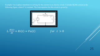
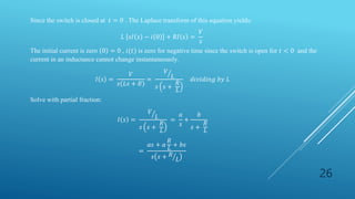
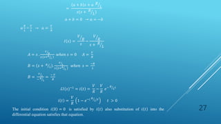
- Example:
Find the Laplace transform for 𝑓 𝑡 = 0
∞
𝑠𝑖𝑛𝑡. 𝑑𝑡
By integration the sine the result will be cosine and have the Laplace
𝑠
𝑠2+1
By using the Laplace transform properties, the result will be ℒ
1
𝑠2+1
Then the Laplace transform for integration the sine is
1
𝑠2+1
𝑠
Which leads the result to
𝑠
𝑠2+1

34. 34
8.Initial Value Theorem
The initial value 𝑓(0) of the function 𝑓(𝑡) whose L.T is 𝑓(𝑠) is:
𝑓 0 = lim
𝑡→0
𝑓(𝑡) = lim
𝑠→∞
𝑠𝑓(𝑠)
- Example: For the function 𝑓 𝑡 = 3𝑒−2𝑡, prove the initial – value theorem:
ℒ3𝑒−2𝑡 =
3
𝑠2 + 2
𝑓 0 = lim
𝑡→0
3𝑒−2𝑡 = lim
𝑠→∞
𝑠
3
𝑠2 + 2
3 = 3
According to Lobital rule in limits that states when there is
∞
∞
then the limit is taking the
derivative of the function of both the nominators and denominators which is in this case
3
1

35. 35
9. Final value theorem:
The final value of the function 𝑓(𝑡) whose L.T is𝑓 ∞ =
lim
𝑡→∞
𝑓(𝑡) = lim
𝑠→0
𝑠𝑓(𝑠)
- Example: For the function 𝑓 𝑡 = 3𝑒−2𝑡
, prove the final –
value theorem:
𝑓 ∞ = lim
𝑡→∞
3𝑒−2𝑡 = lim
𝑠→0
𝑠
3
𝑠2 + 2
0 = 0

36. THANK YOU
36