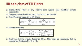
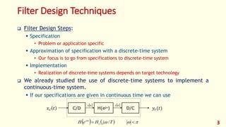
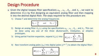
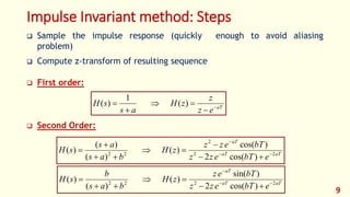
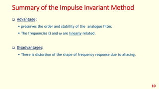
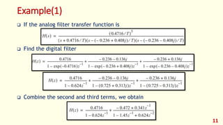
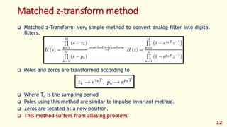
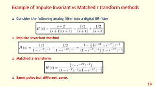
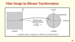
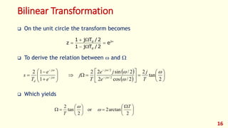
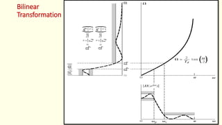
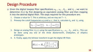
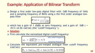
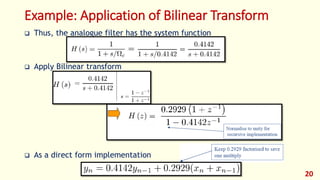
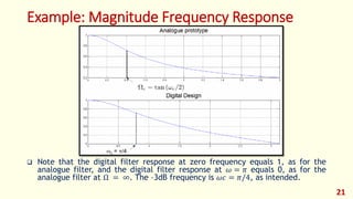
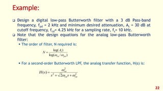
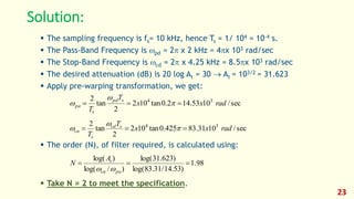
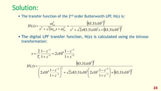
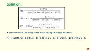
The document discusses the design of discrete-time IIR filters from continuous-time filter specifications. It covers common IIR filter design techniques including the impulse invariance method, matched z-transform method, and bilinear transformation method. An example applies the bilinear transformation to design a first-order low-pass digital filter from a continuous analog prototype. Filter design procedures and steps are provided.

1. ‫ر‬َ‫ـد‬ْ‫ق‬‫ِـ‬‫ن‬،،،‫لما‬‫اننا‬ ‫نصدق‬ْْ‫ق‬ِ‫ن‬‫ر‬َ‫د‬
LECTURE (7)
Discrete-Time IIR Filter Design from
Continuous-Time Filters
Assist. Prof. Amr E. Mohamed

2. IIR as a class of LTI Filters
 Discrete-time Filter is any discrete-time system that modifies certain
frequencies.
 Frequency-selective filters pass only certain frequencies
 The difference equation of IIR filters:
 Transfer function:
 To give an Infinite Impulse Response (IIR), a filter must be recursive, that is,
incorporate feedback N ≠ 0, M ≠ 0.
2

3. 3
Filter Design Techniques
 Filter Design Steps:
 Specification
• Problem or application specific
 Approximation of specification with a discrete-time system
• Our focus is to go from specifications to discrete-time system
 Implementation
• Realization of discrete-time systems depends on target technology
 We already studied the use of discrete-time systems to implement a
continuous-time system.
 If our specifications are given in continuous time we can use
D/C𝑥 𝑐 𝑡 𝑦𝑟(𝑡)C/D H(ej)
 nx  ny
    
 /TjHeH c
j

4. Filter Specifications
 Specifications
 Passband
 Stopband
 Parameters
 Specifications in dB
 Ideal passband 𝑔𝑎𝑖𝑛 = 20log(1) = 0 𝑑𝐵
 Max passband 𝑔𝑎𝑖𝑛 = 20log(1.01) = 0.086𝑑𝐵
 Max stopband 𝑔𝑎𝑖𝑛 = 20log(0.001) = −60 𝑑𝐵
4
   20002001.199.0  forjHeff
     30002001.0 forjHeff
 
 30002
20002
001.0
01.0
2
1








s
p

5. Design of IIR Filters
 A digital filter, , with infinite impulse response (IIR), can be designed
by first transforming it into a prototype analog filter and then design
this analog filter using a standard procedure.
 Once the analog filter is properly designed, it is then mapped back to the
discrete-time domain to obtain a digital filter that meets the specifications.
5
)( jw
eH
)( jHc

6. Design of IIR Filters
 The commonly used analog filters are
1. Butterworth filters: no ripples at all,
2. Chebyshev filters: ripples in the passband OR in the stopband, and
3. Elliptical filters: ripples in BOTH the pass and stop bands.
 A disadvantage of IIR filters is that they usually have nonlinear phase.
Some minor signal distortion is a result.
 There are two main techniques used to design IIR filters:
1. The Impulse Invariant method,
2. Matched z-transform method, and
3. The Bilinear transformation method.
6

7. 7
Filter Design by Impulse Invariance
 In this design method we want the digital filter impulse response to look “similar”
to that of a frequency-selective analog filter. Hence we sample ℎ 𝑎(𝑡) at some
sampling interval T to obtain h(n); that is,
 Mapping a continuous-time impulse response to discrete-time
 Mapping a continuous-time frequency response to discrete-time
 The analog and digital frequencies are related by 𝜔 = Ω𝑇 𝑜𝑟 𝑒 𝑗𝜔 = 𝑒 𝑗Ω𝑇 𝑜𝑟 𝑧 = 𝑒 𝑠𝑇
 If the continuous-time filter is band-limited to
   nThnh c
  









k
c
j
k
T
j
T
jH
T
eH
 21
  








1
d
c
j
T
jH
T
eH
  dc TjH /for0 

8. Design Procedure
 Given the digital lowpass filter specifications 𝜔 𝑝 , 𝜔𝑠 , 𝑅 𝑝 , and 𝐴 𝑠 , we want to
determine 𝐻(𝑧) by first designing an equivalent analog filter and then mapping
it into the desired digital filter. The steps required for this procedure are:
1) Choose T and determine the analog frequencies
2) Design an analog filter 𝐻 𝑎(𝑠) using the specifications 𝜔 𝑝 , 𝜔𝑠 , 𝑅 𝑝 , and 𝐴 𝑠. This can
be done using any one of the three (Butterworth, Chebyshev, or elliptic)
prototypes.
3) Using partial fraction expansion, expand 𝐻 𝑎(𝑠) into
4) Now transform analog poles {𝑝 𝑘} into digital poles {𝑒 𝑝 𝑘 𝑇} to obtain the digital filter:
8

9. 9
Impulse Invariant method: Steps
 Sample the impulse response (quickly enough to avoid aliasing
problem)
 Compute z-transform of resulting sequence
 First order:
 Second Order:
aT
ez
z
zH
as
sH 



 )(
1
)(
aTaT
aT
ebTezz
bTezz
zH
bas
as
sH 22
2
22
)cos(2
)cos(
)(
)(
)(
)( 







aTaT
aT
ebTezz
bTez
zH
bas
b
sH 2222
)cos(2
)sin(
)(
)(
)( 






10. 10
Summary of the Impulse Invariant Method
 Advantage:
 preserves the order and stability of the analogue filter.
 The frequencies Ω and ω are linearly related.
 Disadvantages:
 There is distortion of the shape of frequency response due to aliasing.

11. Example(1)
 If the analog filter transfer function is
 Find the digital filter
 Combine the second and third terms, we obtain
11

12. Matched z-transform method
 Matched z-Transform: very simple method to convert analog filter into digital
filters.
 Poles and zeros are transformed according to
 Where Td is the sampling period
 Poles using this method are similar to impulse invariant method.
 Zeros are located at a new position.
 This method suffers from aliasing problem.
12

13. 13
Example of Impulse Invariant vs Matched z transform methods
 Consider the following analog filter into a digital IIR filter
 Impulse invariant method
 Matched z-transform
 Same poles but different zeros

14. 14
Filter Design by Bilinear Transformation
 Get around the aliasing problem of impulse invariance
 Map the entire s-plane onto the unit-circle in the z-plane
 Nonlinear transformation
 Frequency response subject to warping
 Bilinear transformation
 Transformed system function
 Again T cancels out so we can ignore it
 We can solve the transformation for z as
 Maps the left-half s-plane into the inside of the unit-circle in z
 Stable in one domain would stay in the other








 

1
1
1
12
z
z
T
s
  













 

1
1
1
12
z
z
T
HzH c
 
  2/2/1
2/2/1
2/1
2/1
TjT
TjT
sT
sT
z








 js

15. 15
Filter Design by Bilinear Transformation

16. 16
Bilinear Transformation
 On the unit circle the transform becomes
 To derive the relation between  and 
 Which yields




 j
d
d
e
2/Tj1
2/Tj1
z
 
 




















 



2
tan
2
2/cos2
2/sin22
1
12
2/
2/







T
j
e
je
T
j
e
e
T
s j
j
j
j
d





 







2
arctan2or
2
tan
2 T
T



17. 17
Bilinear
Transformation

18. Design Procedure
 Given the digital lowpass filter specifications 𝜔 𝑝 , 𝜔𝑠 , 𝑅 𝑝 , and 𝐴 𝑠 , we want to
determine 𝐻(𝑧) by first designing an equivalent analog filter and then mapping
it into the desired digital filter. The steps required for this procedure are:
1. Choose a value for T. This is arbitrary, and we may set T = 1.
2. Prewarp the cutoff frequencies ω p and ω s ; that is, calculate Ω 𝑝 and Ω 𝑠 using.
3. Design an analog filter 𝐻 𝑎(𝑠) using the specifications 𝜔 𝑝 , 𝜔𝑠 , 𝑅 𝑝 , and 𝐴 𝑠. This can
be done using any one of the three (Butterworth, Chebyshev, or elliptic)
prototypes.
4. 4. finally, apply the bilinear transform to get the digital IIR filter.
18

19. Example: Application of Bilinear Transform
 Design a first order low-pass digital filter with -3dB frequency of 1kHz
and a sampling frequency of 8kHz using a the first order analogue low-
pass filter
 which has a gain of 1 (0dB) at zero frequency, and a gain of -3dB ( =
√0.5 ) at Ωc rad/sec (the "cutoff frequency ").
 Solution:
 First calculate the normalized digital cutoff frequency:
 Calculate the equivalent pre-warped analogue filter cutoff frequency
(rad/sec)
19

20. Example: Application of Bilinear Transform
 Thus, the analogue filter has the system function
 Apply Bilinear transform
 As a direct form implementation
20

21. Example: Magnitude Frequency Response
 Note that the digital filter response at zero frequency equals 1, as for the
analogue filter, and the digital filter response at 𝜔 = 𝜋 equals 0, as for the
analogue filter at Ω = ∞. The –3dB frequency is 𝜔𝑐 = 𝜋/4, as intended.
21

22. Example:
 Design a digital low-pass Butterworth filter with a 3 dB Pass-band
frequency, fpd = 2 kHz and minimum desired attenuation, At = 30 dB at
cutoff frequency, fcd= 4.25 kHz for a sampling rate, fs= 10 kHz.
 Note that the design equations for the analog low-pass Butterworth
filter:
 The order of filter, N required is:
 For a second-order Butterworth LPF, the analog transfer function, H(s) is:
22
)/log(
)log(
paca
tA
N


22
2
2
)(
caca
ca
ss
sH





23. Solution:
 The sampling frequency is fs= 10 kHz, hence Ts = 1/ 104 = 10-4 s.
 The Pass-Band Frequency is pd = 2 x 2 kHz = 4x 103 rad/sec
 The Stop-Band Frequency is cd = 2 x 4.25 kHz = 8.5x 103 rad/sec
 The desired attenuation (dB) is 20 log At = 30  At = 103/2 = 31.623
 Apply pre-warping transformation, we get:
 The order (N), of filter required, is calculated using:
 Take N = 2 to meet the specification.
23
sec/1053.142.0tan102
2
tan
2 34
radxx
T
T
spd
s
pa  


sec/1031.83425.0tan102
2
tan
2 34
radxx
T
T
scd
s
ca  


98.1
)53.14/31.83log(
)623.31log(
)/log(
)log(

paca
tA
N


24. Solution:
 The transfer function of the 2nd order Butterworth LPF, H(s) is:
 The digital LPF transfer function, H(z) is calculated using the bilinear
transformation:
24
 
 2332
23
22
2
1031.831031.832
1031.83
2
)(
xsxxs
x
ss
sH
caca
ca






1
1
4
1
1
1
1
102
1
12










z
z
x
z
z
T
s
s
 
 23
1
1
33
2
1
1
4
23
1031.83
1
1
1021031.832
1
1
102
1031.83
)(
x
z
z
xxx
z
z
x
x
zH






















25. Solution:
 From which we can finally write the following difference equation:
𝒀 𝒏 = 𝟎. 𝟐𝟎𝟔𝟓𝟕 𝒙 𝒏 + 𝟎. 𝟒𝟏𝟑𝟏 𝒙(𝒏 − 𝟏) + 𝟎. 𝟐𝟎(𝟔𝟓𝟕 𝒙(𝒏 − 𝟐) + 𝟎. 𝟑𝟔𝟗𝟓𝟑 𝒚(𝒏 − 𝟏)– 𝟎. 𝟏𝟗𝟓𝟖𝟐 𝒚(𝒏 − 𝟐)
25

26. Solution:
 In order to check the magnitude characteristics of the frequency response,
rewrite:
 DC-gain: Ts = 0  z = 1 which gives |H(z)| =1
 3-dB cut-off frequency : pd Ts = 0.4
 We can also check the 30dB minimum attenuation requirement by working out
H(ej0.85j)
26

27. 27