Downloaded 426 times

![>> n=0:20;
>> omega=pi/4; % This is the cut-off frequency
>> h=(omega/pi)*sinc(omega*(n-10)/pi); % Note the 10 step shift
>> stem(n,h)
>> title('Sample-Shifted LP Impulse Response')
>> xlabel('n')
>> ylabel('h[n]')
>> fvtool(h,1)
0 2 4 6 8 10 12 14 16 18 20
-0.1
-0.05
0
0.05
0.1
0.15
0.2
0.25
Sample-Shifted LP Impulse Response
n
h[n]
0 0.1 0.2 0.3 0.4 0.5 0.6 0.7 0.8 0.9
0
0.2
0.4
0.6
0.8
1
1.2
1.4
Normalized Frequency ( rad/sample)
Magnitude
Magnitude Response
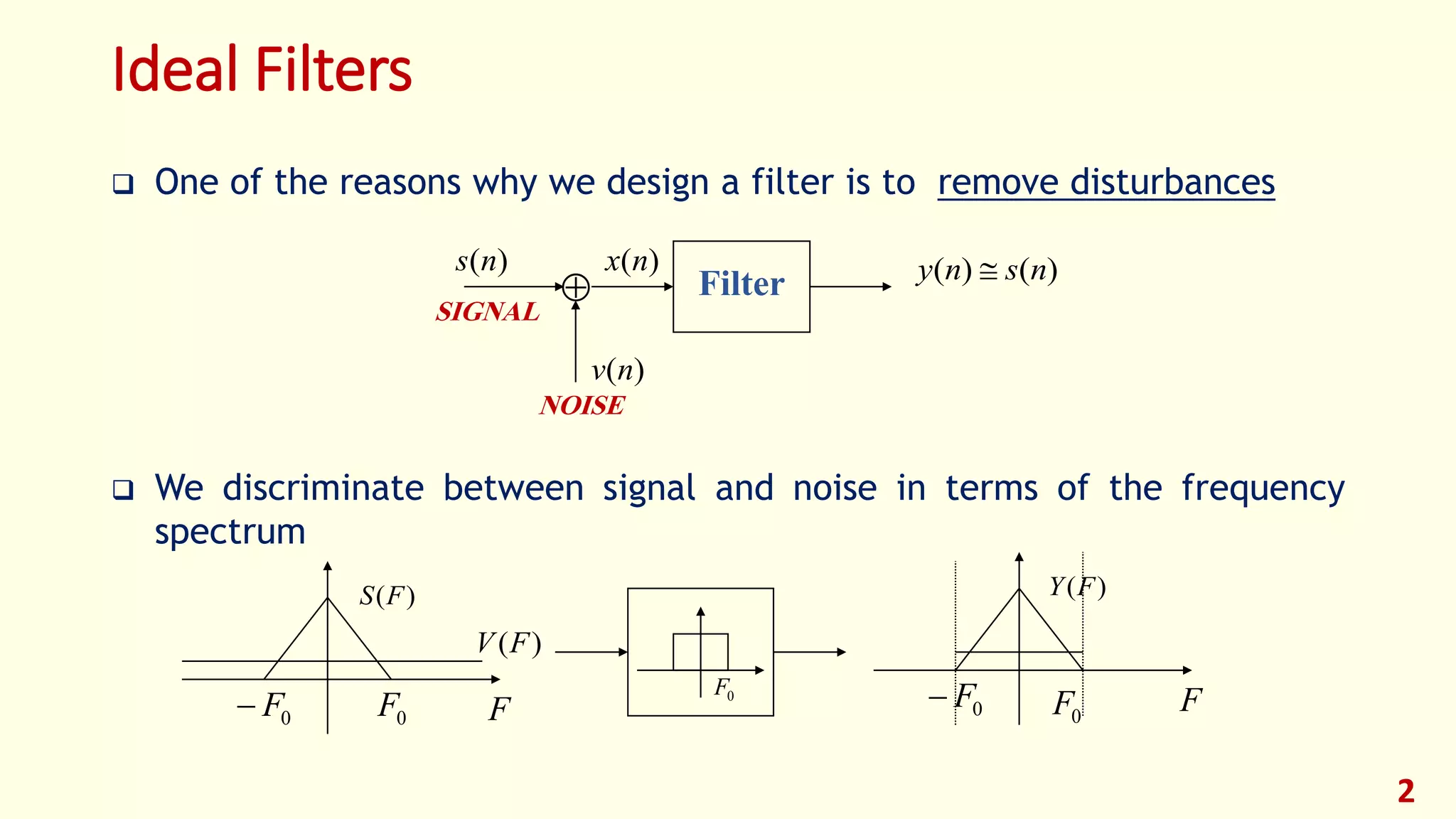
Note the linear phase properties of
the impulse response
Example: 21 Coefficient LP Filter with Ω0 = π/4](https://image.slidesharecdn.com/dsp2018foehu-lec06-firfilterdesign-180425222719/75/DSP_2018_FOEHU-Lec-06-FIR-Filter-Design-15-2048.jpg)
![17
Windowing in Frequency Domain
Windowed frequency response
The windowed version is smeared version of desired response
If w[n]=1 for all n, then W(ej) is pulse train with 2 period
deWeHeH jj
d
j
2
1](https://image.slidesharecdn.com/dsp2018foehu-lec06-firfilterdesign-180425222719/75/DSP_2018_FOEHU-Lec-06-FIR-Filter-Design-17-2048.jpg)
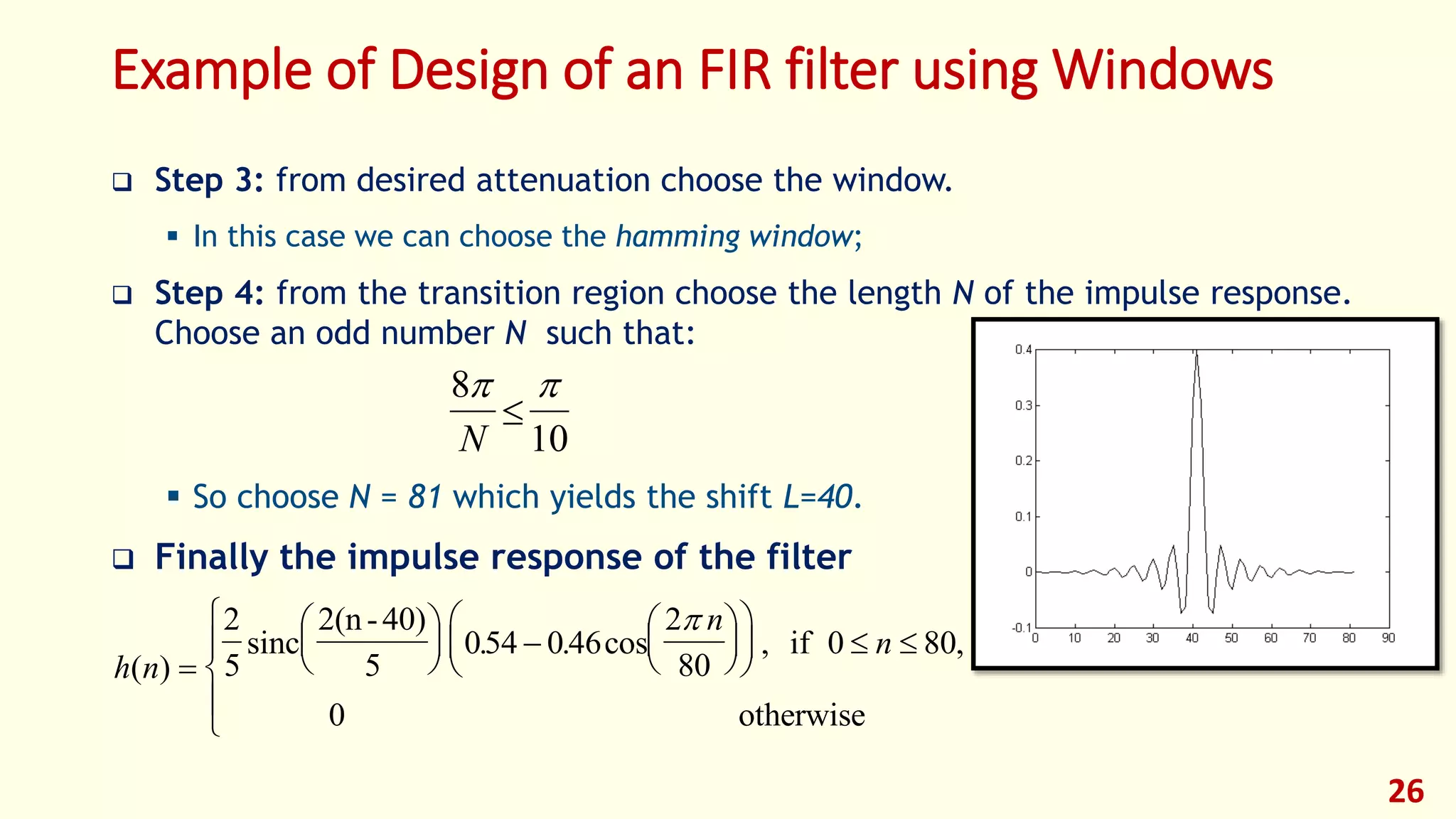
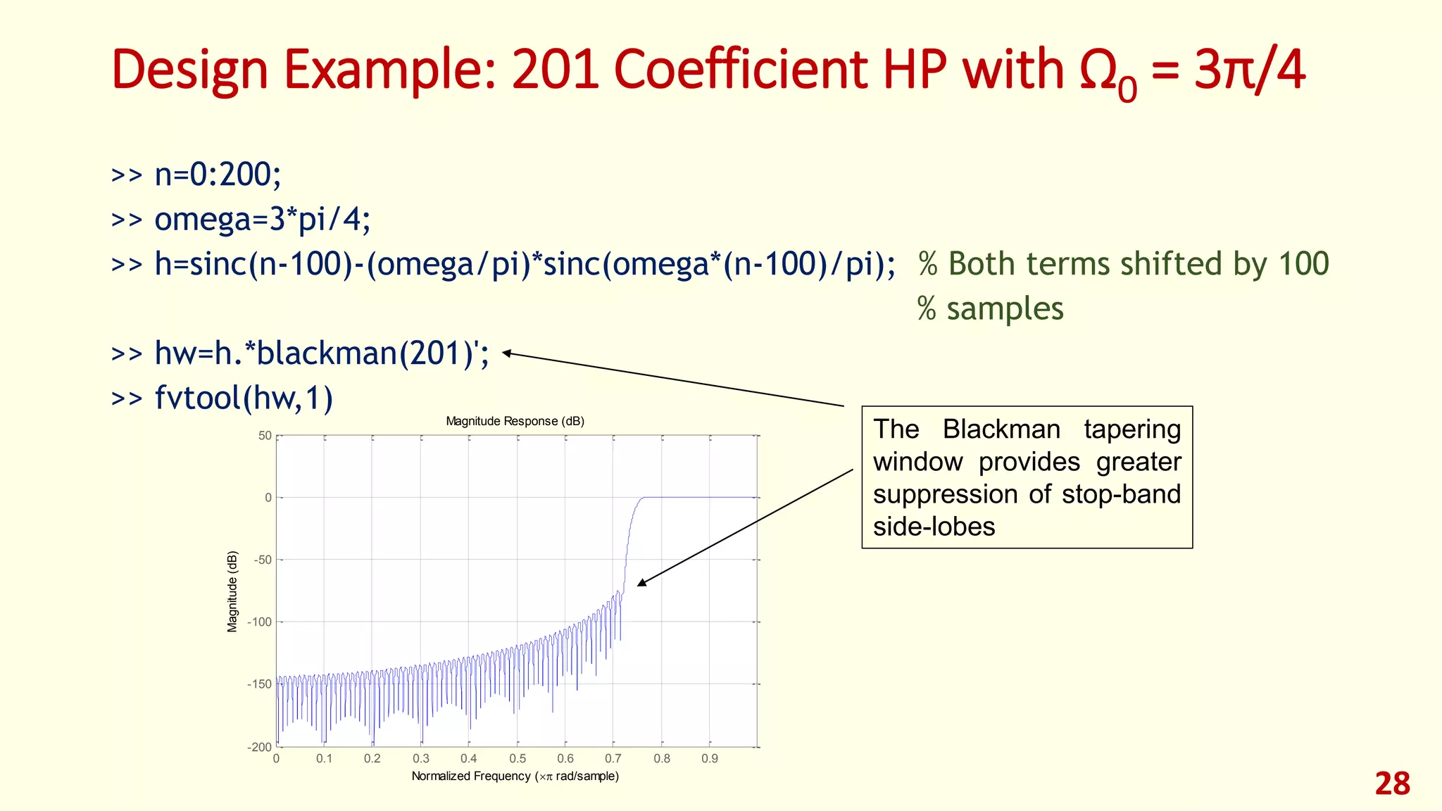


This lecture discusses the design of finite impulse response (FIR) filters. It introduces the window method for FIR filter design, which involves truncating the ideal impulse response with a window function to obtain a causal FIR filter. Common window functions are presented such as rectangular, triangular, Hanning, Hamming, and Blackman windows. These windows trade off main lobe width and side lobe levels. The document provides an example design of a low-pass FIR filter using the Hamming window to meet given passband and stopband specifications.
Introduction to FIR filter design by Assist. Prof. Amr E. Mohamed.
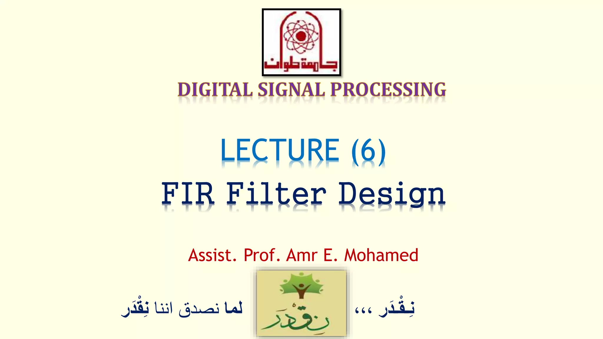
Ideal filters remove disturbances, distinguishing between signal and noise via frequency spectrum.
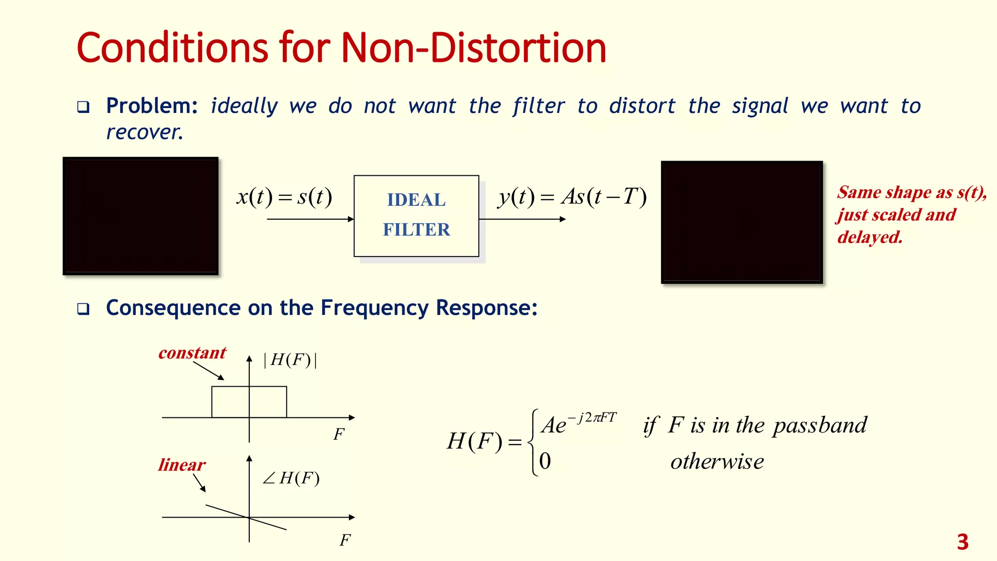
Conditions for non-distortion, focusing on frequency response and ideal filters preserving signal shape.
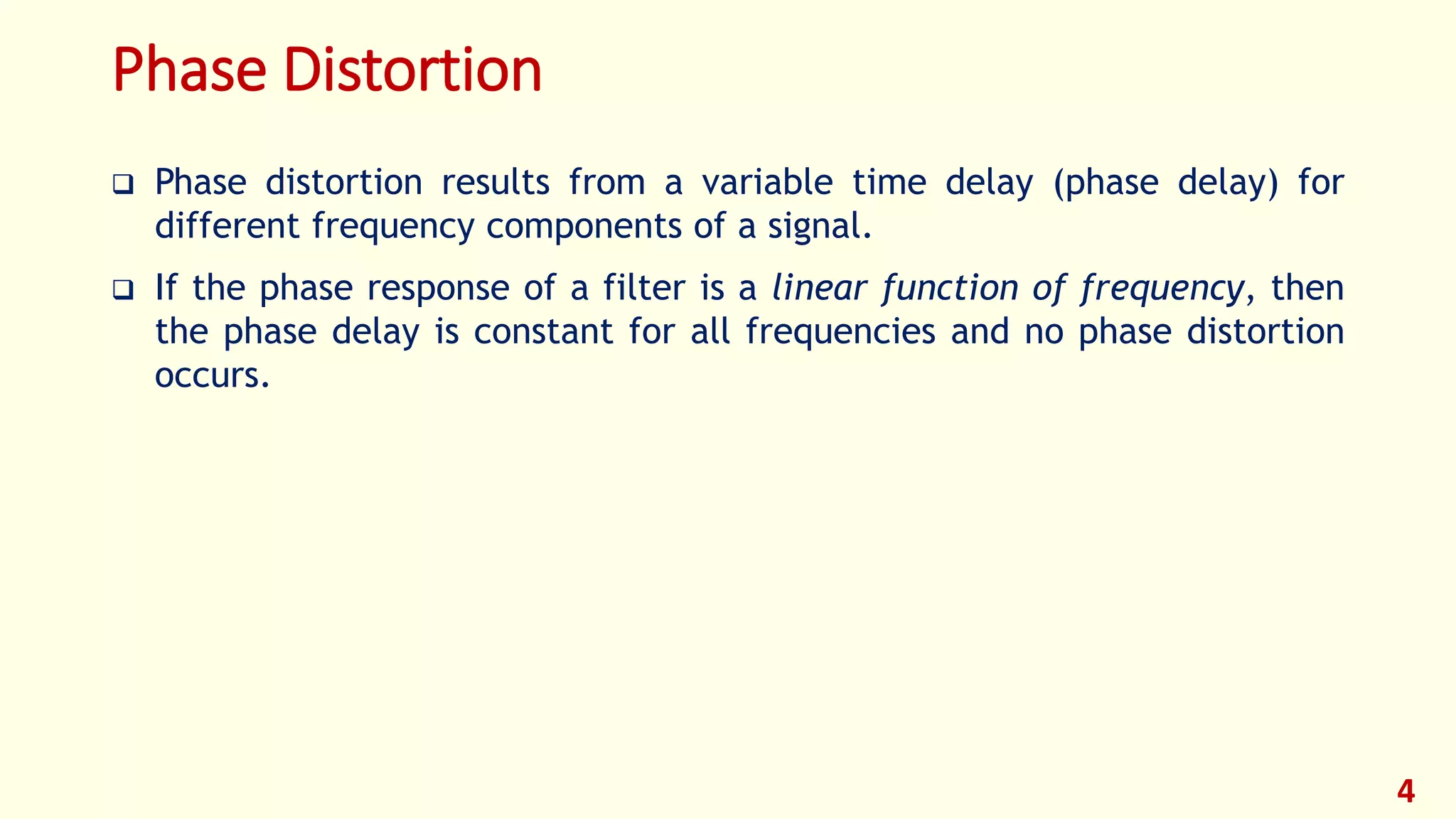
Phase distortion occurs due to variable time delay; linear phase response prevents distortion.
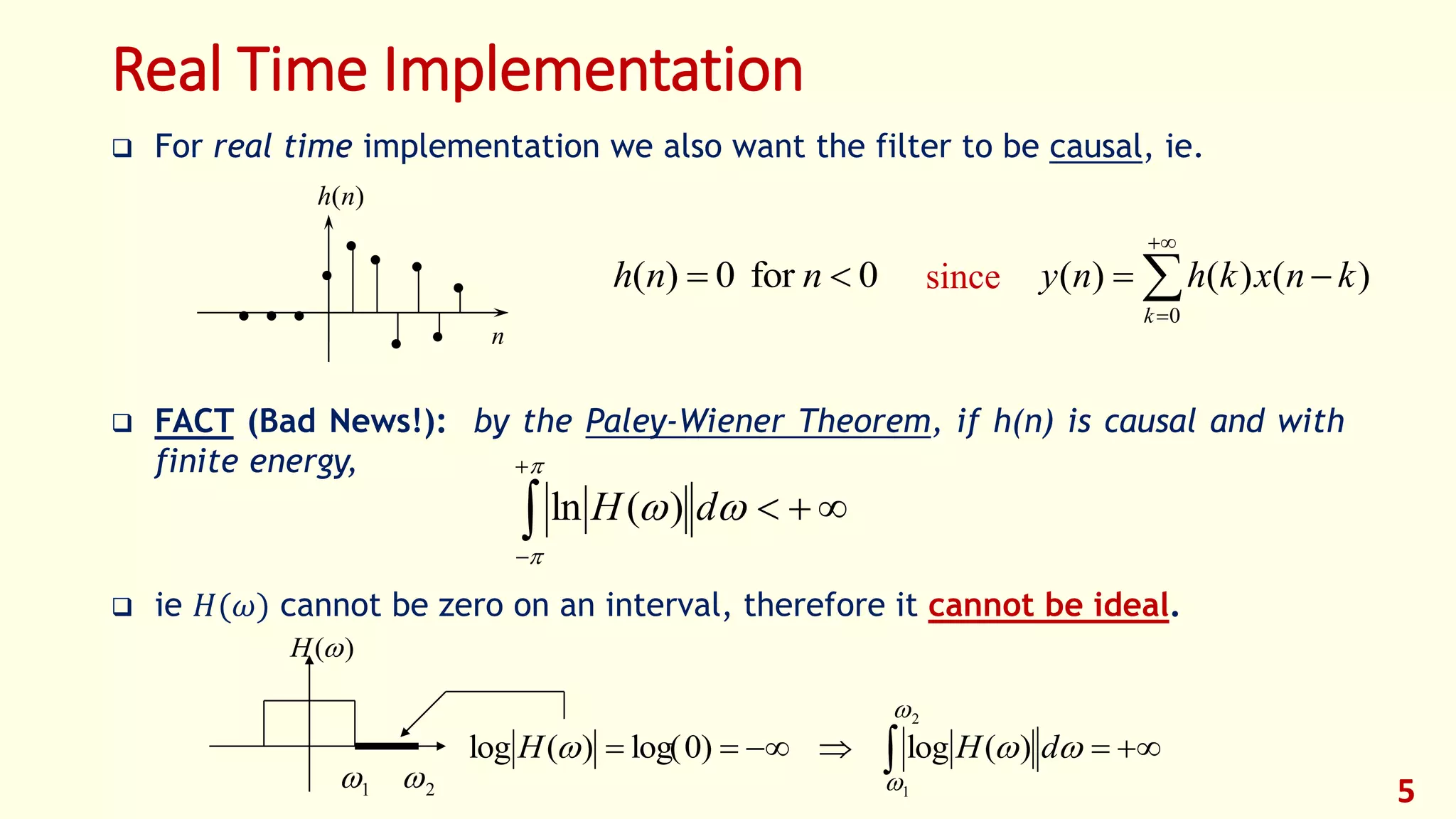
Causal filters are required for real-time implementation; ideal filters are difficult to achieve.
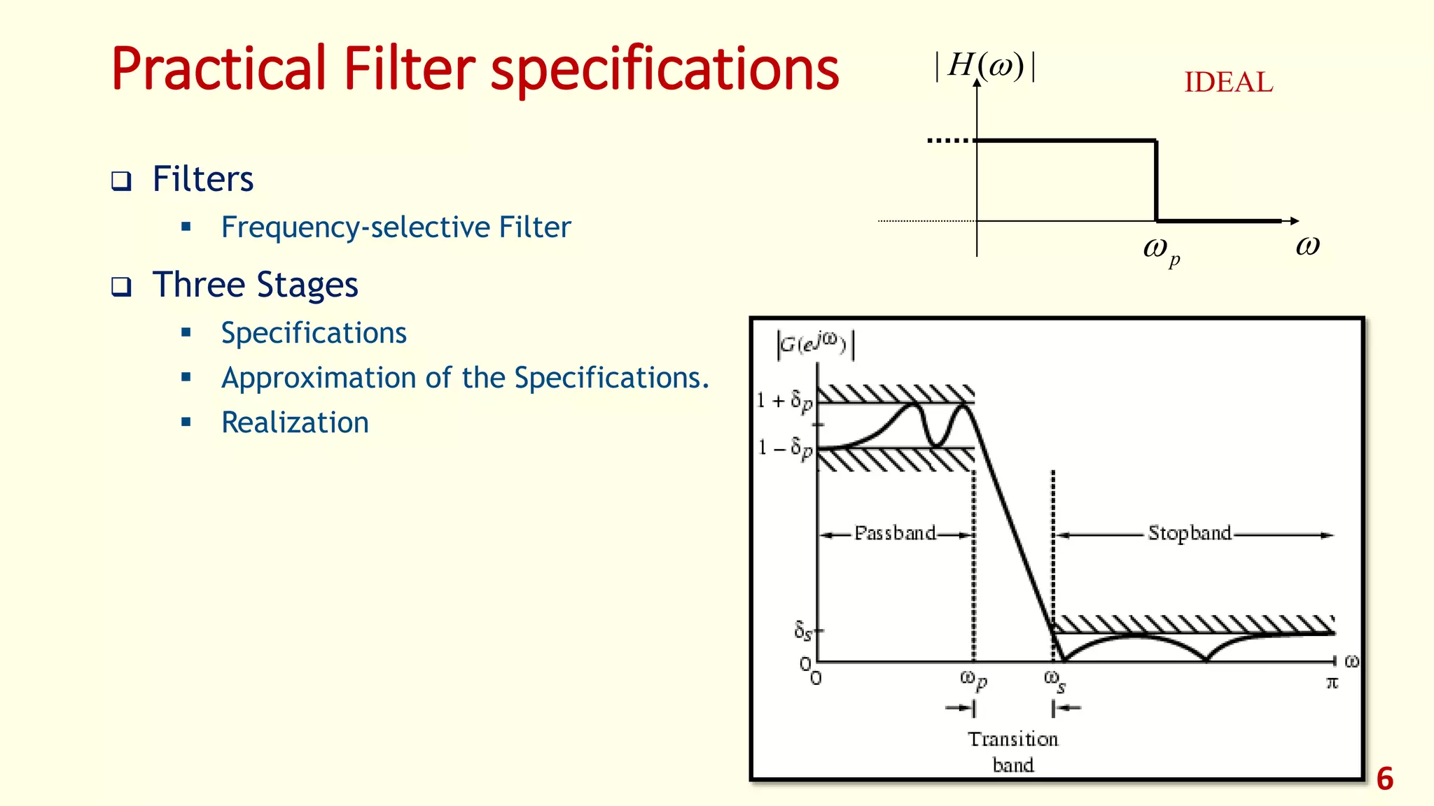
Practical filter specifications include passband/stop-band edge frequency and maximum ripple.
Comparison of FIR filters, characterized by stability and linear phase, with IIR filters being selective.
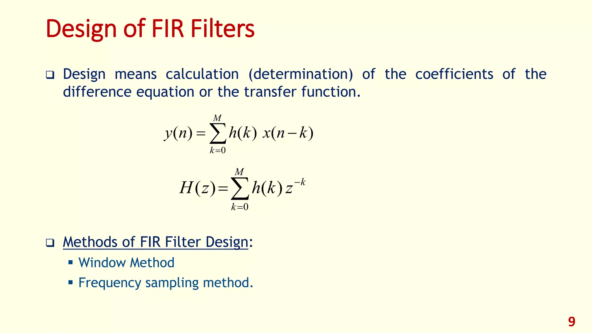
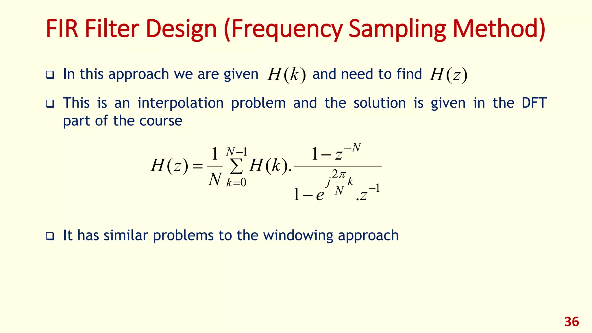
Methods for FIR filter design include the window method and frequency sampling method.
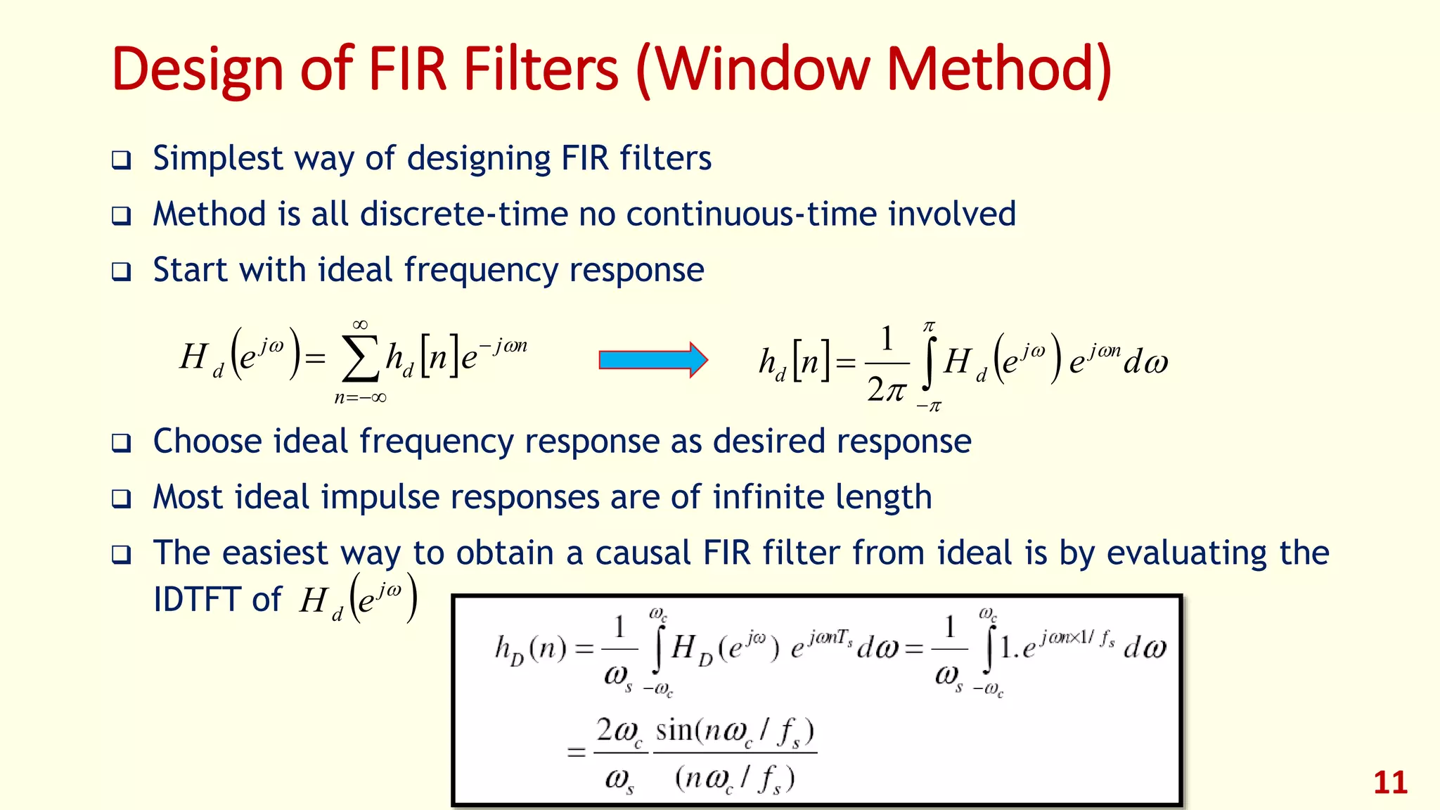
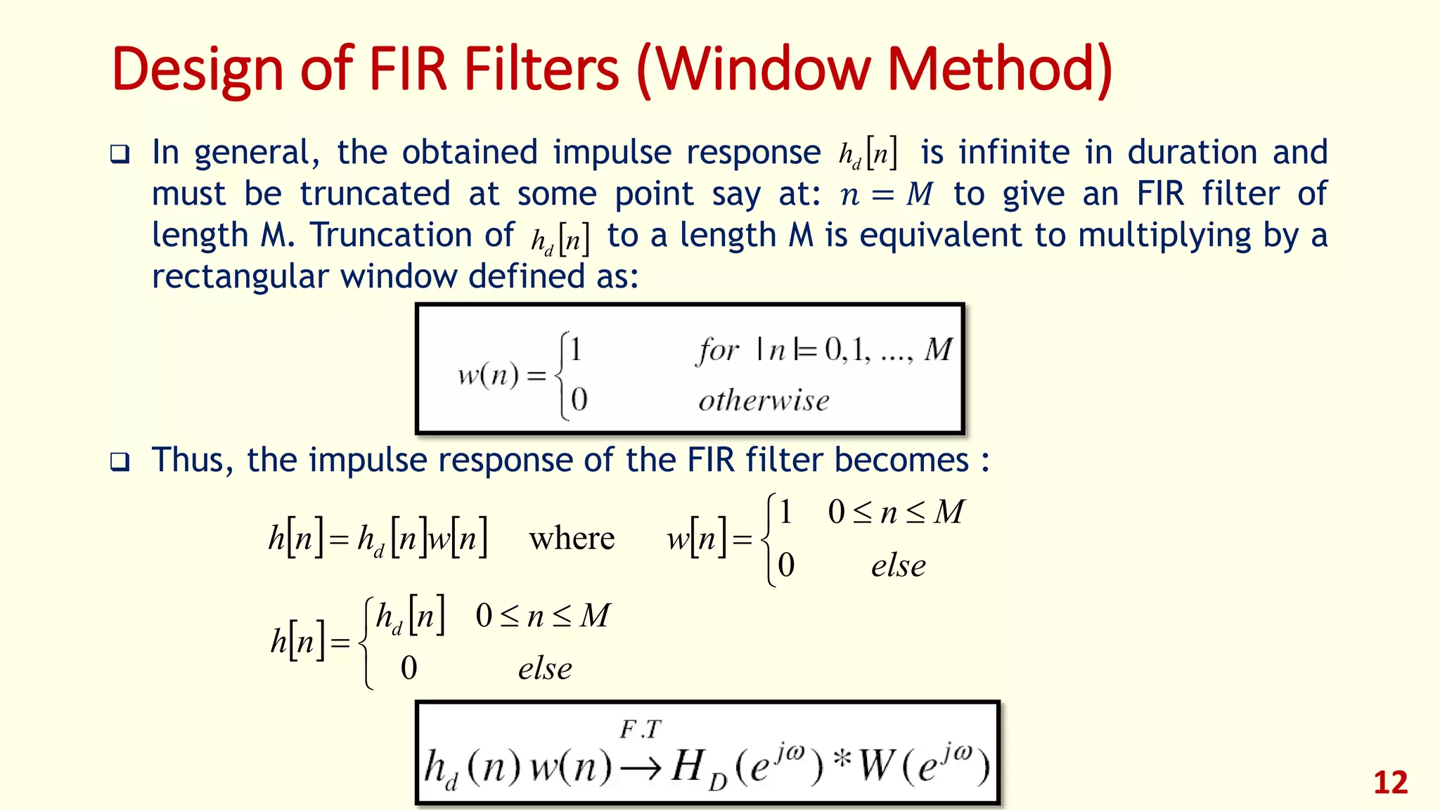
The simplest FIR design method uses ideal frequency response; the impulse response is typically infinite.
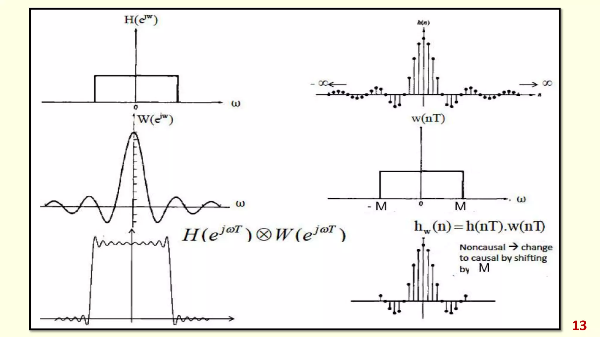
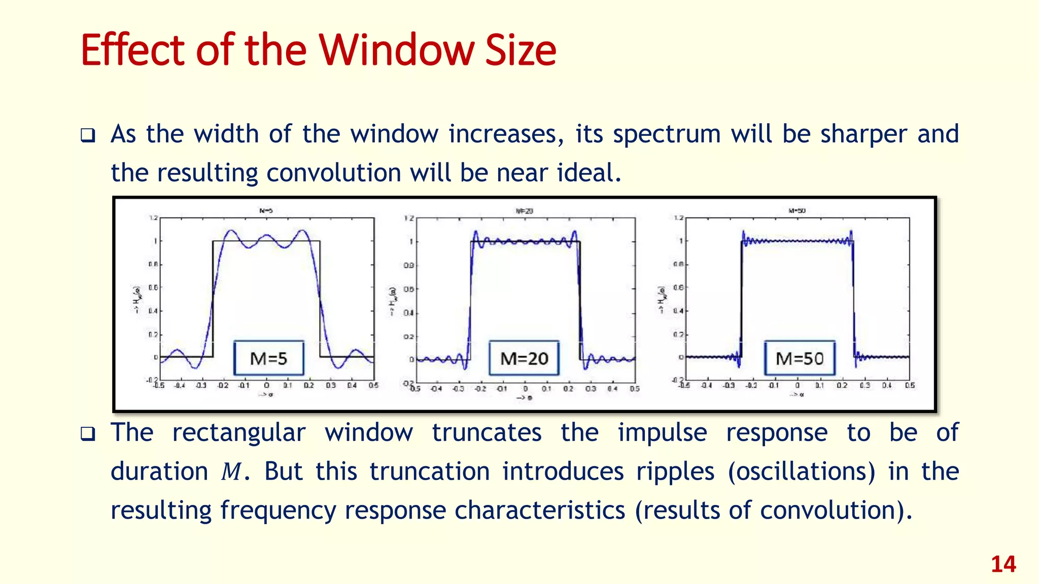
Truncation of impulse responses introduces ripples; window size affects the ideality of the filter.
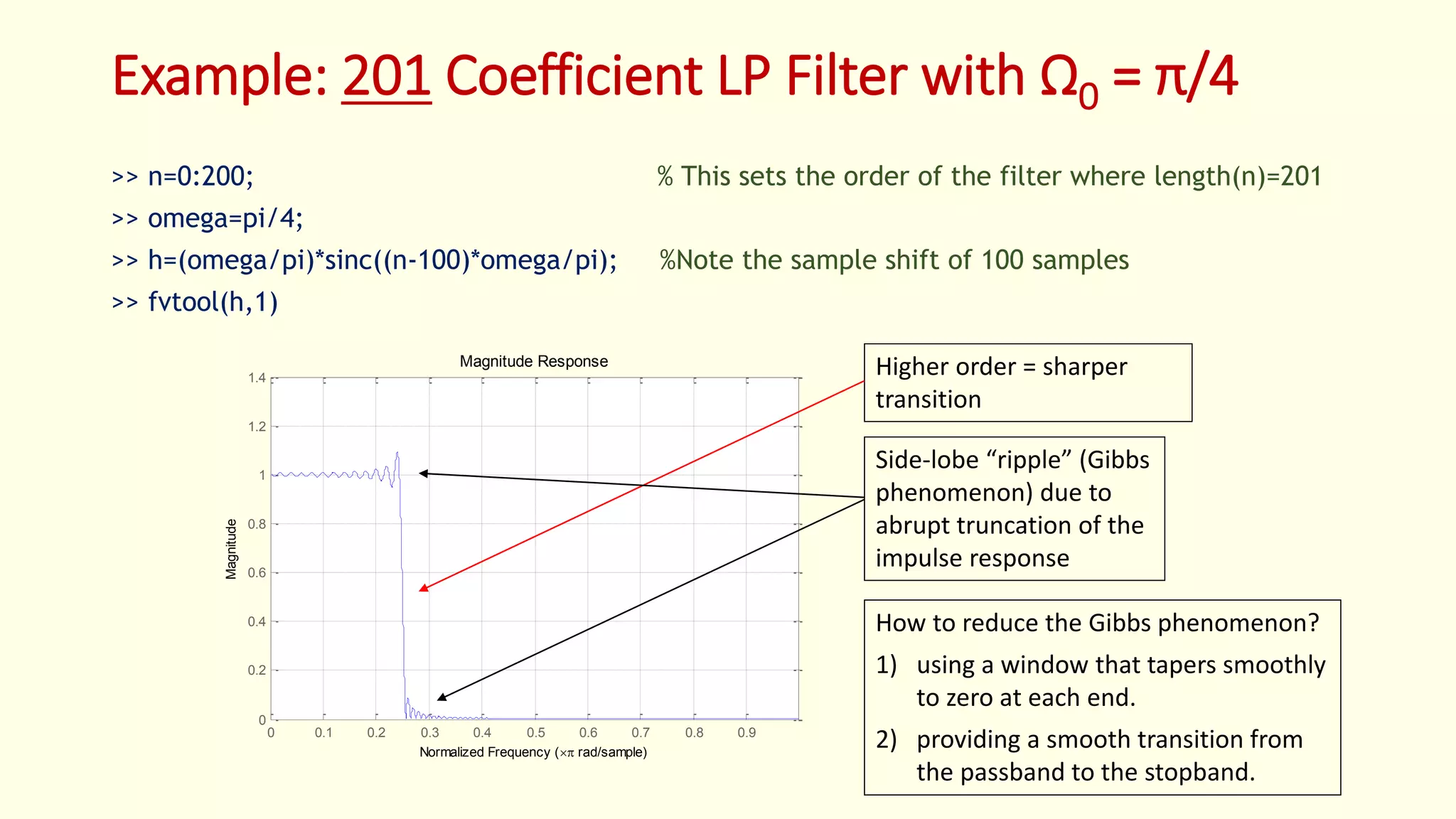
Examples of sample-shifted low-pass filter impulse responses and effects of filter order and Gibbs phenomenon.
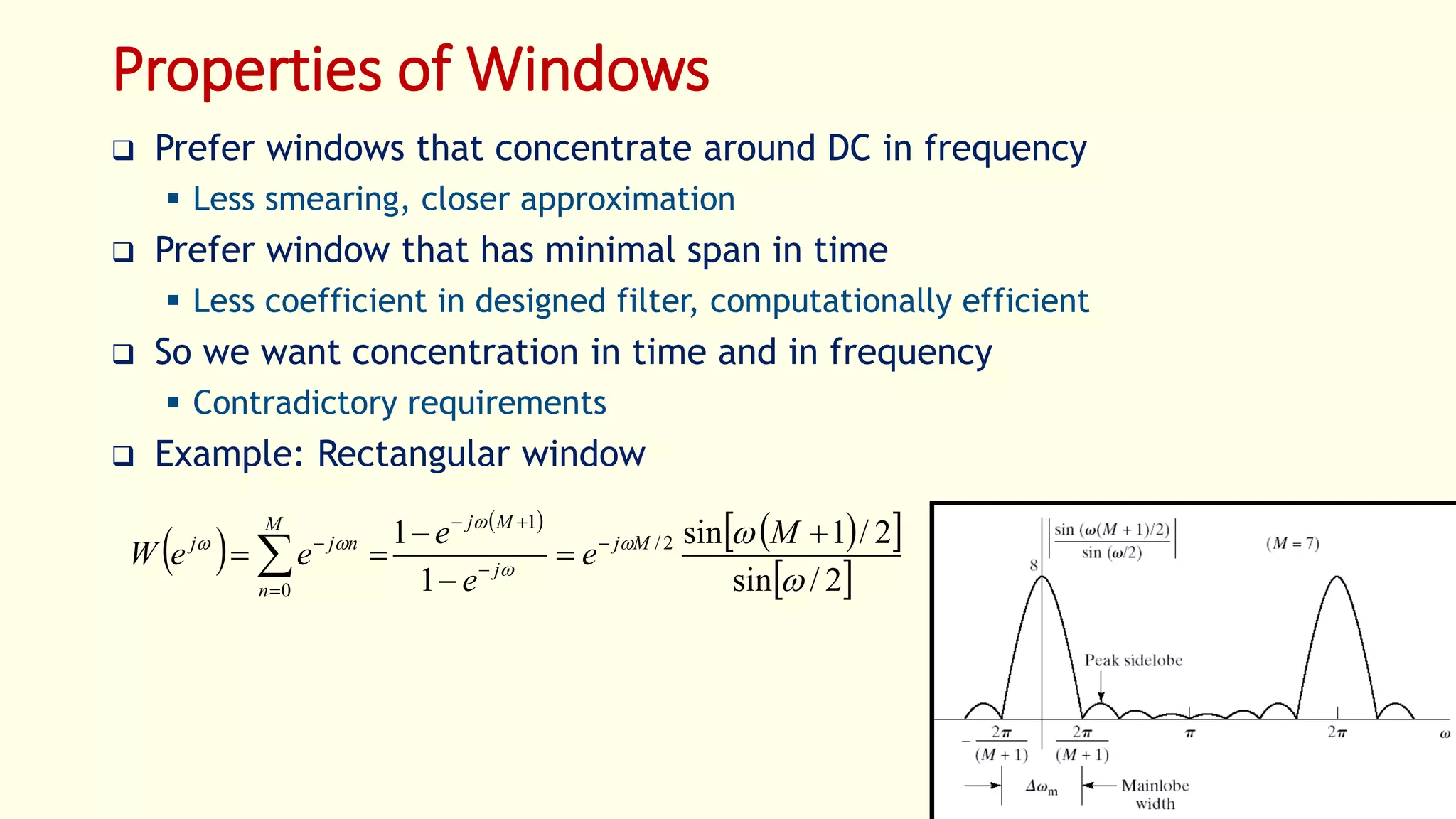
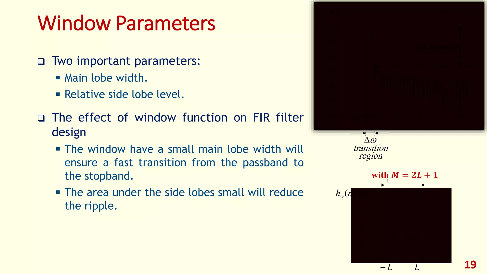
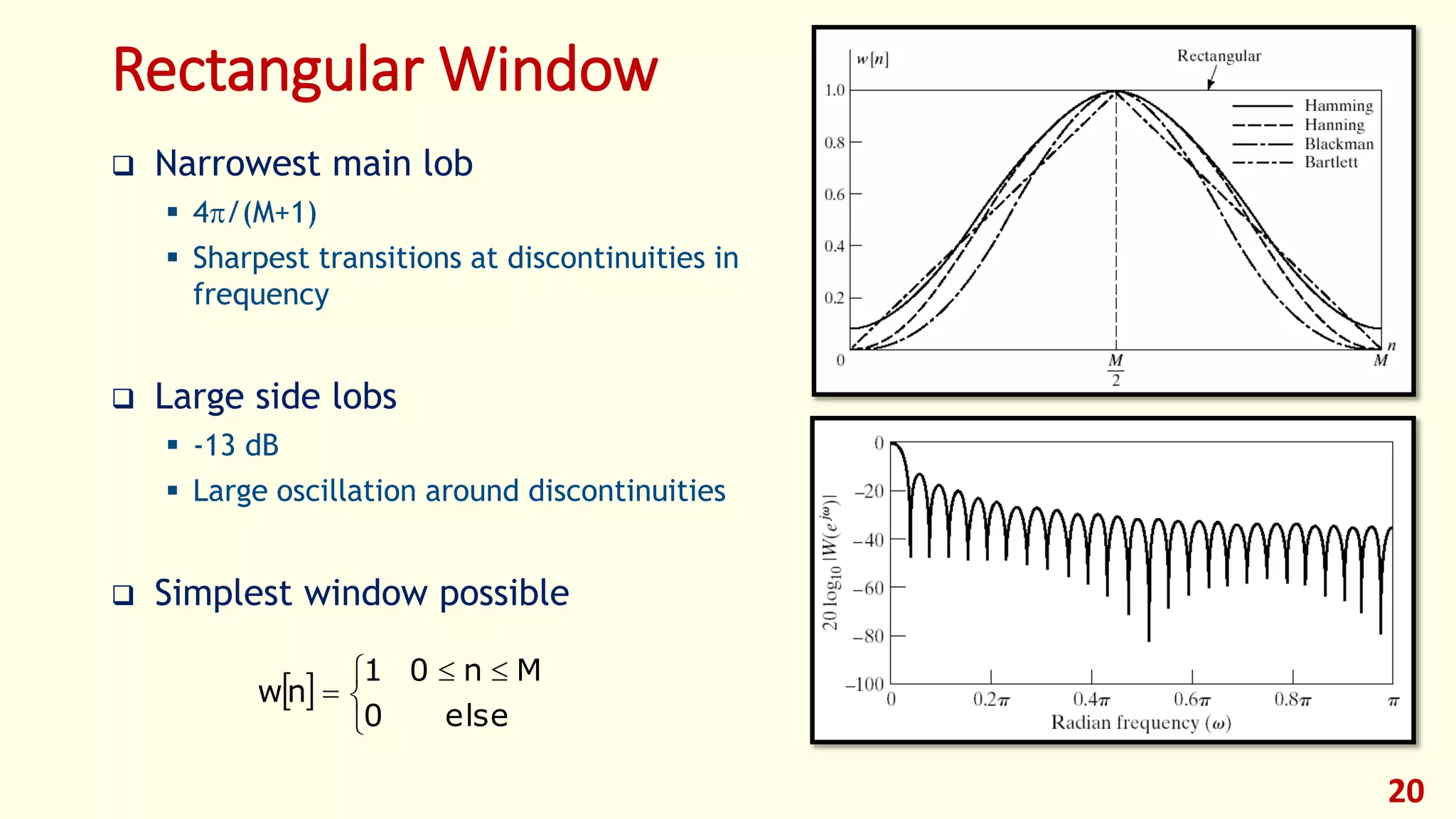
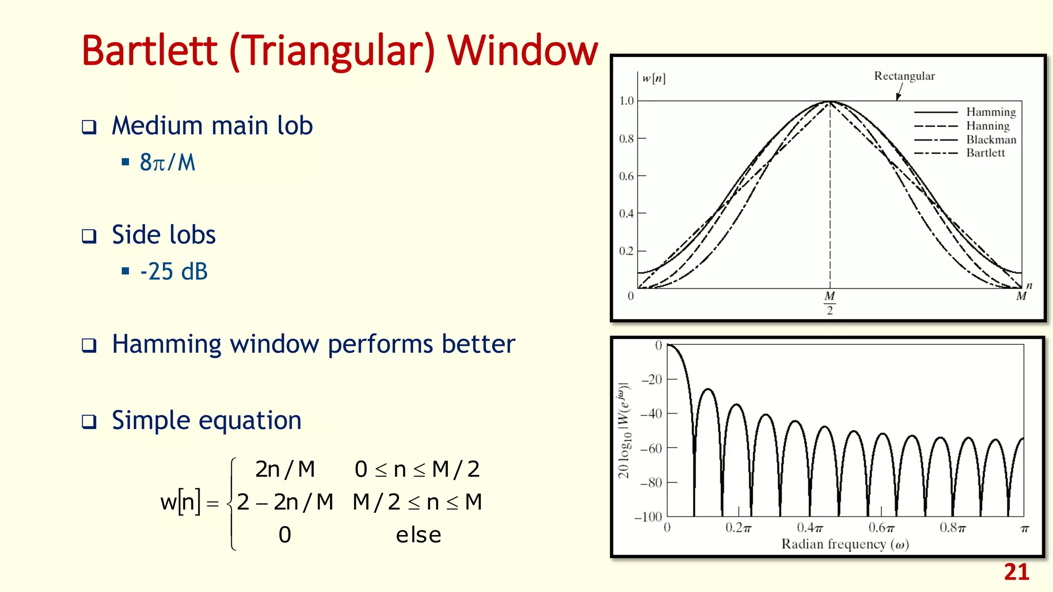
Windowing operations influence frequency response; properties of different window types like rectangular, Bartlett.
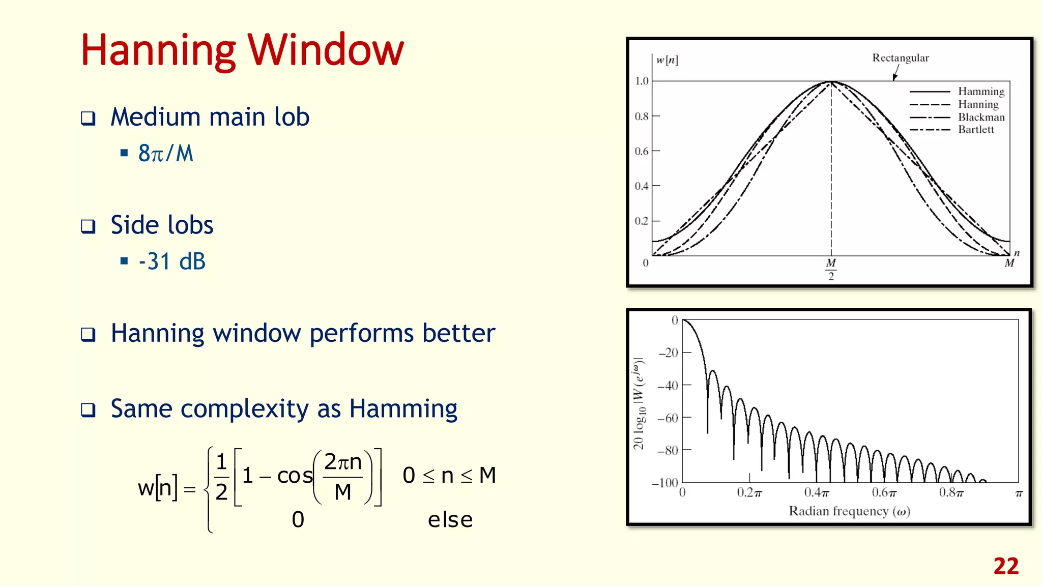
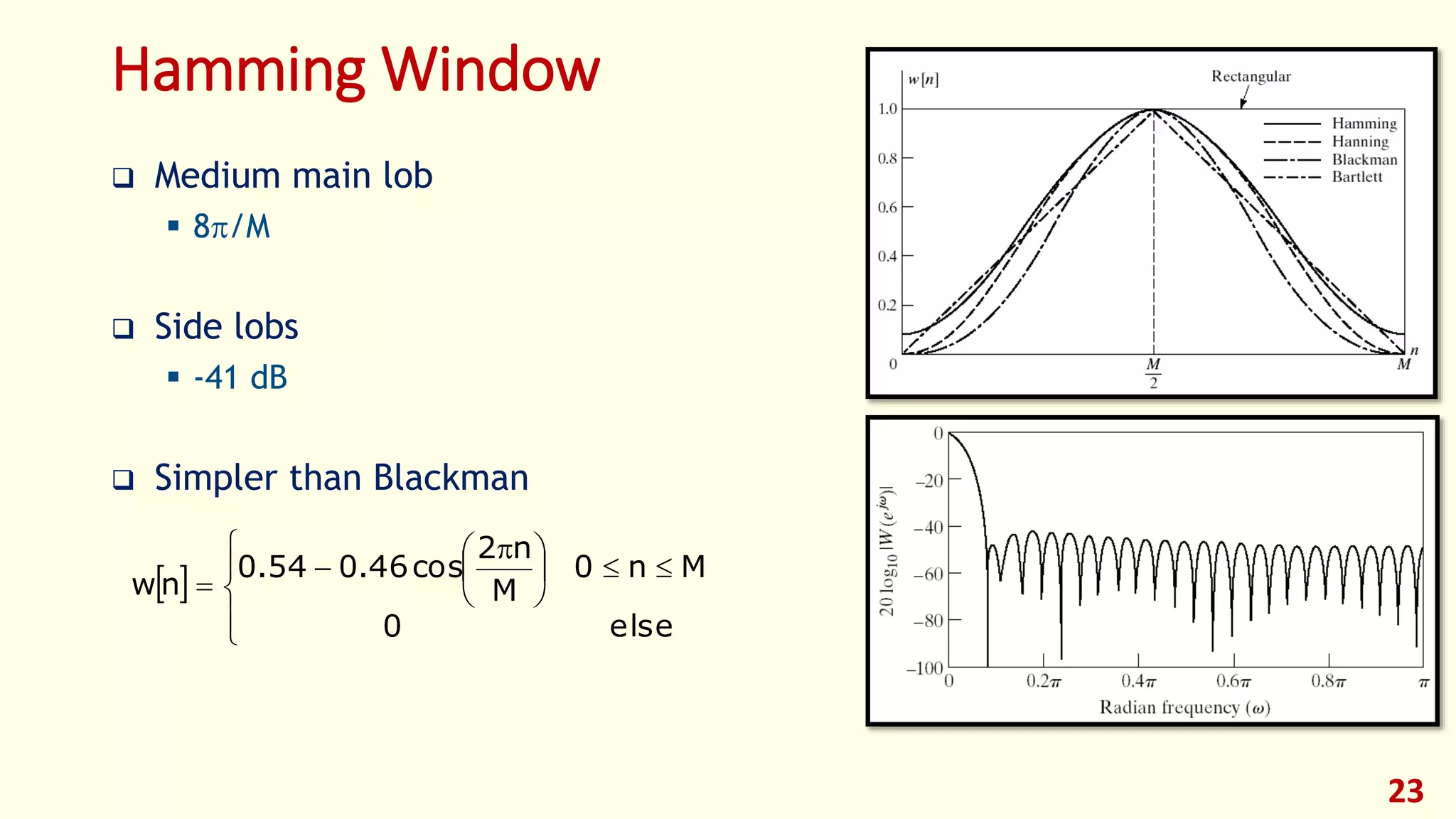
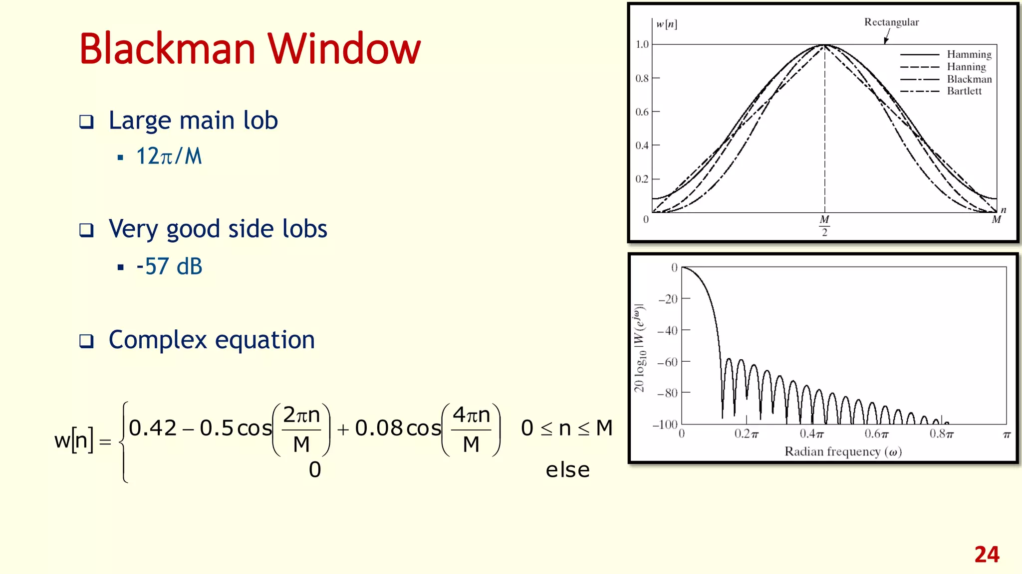
Characteristics of different windows: Bartlett, Hanning, Hamming, and Blackman; side lobe levels vary.
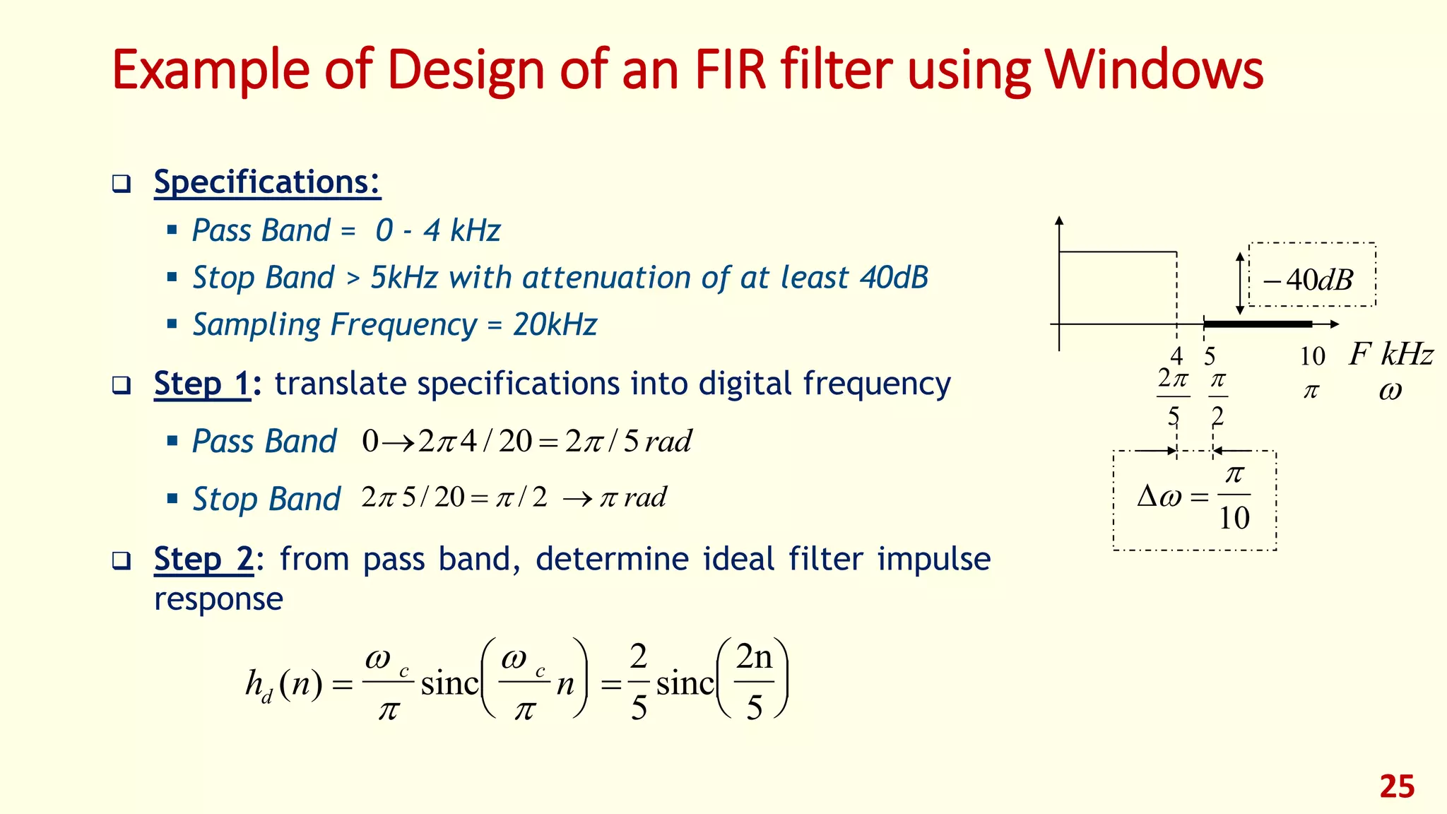
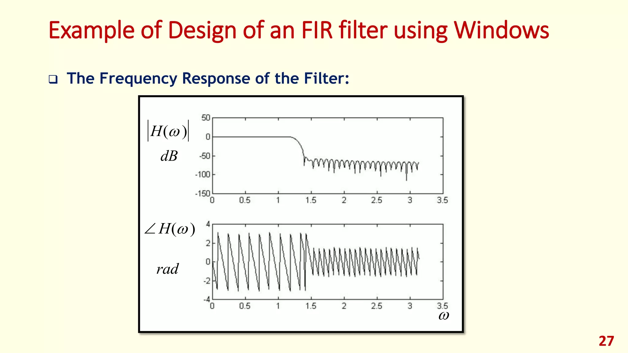
Practical design steps for FIR filters using specified frequencies and selecting appropriate windows.
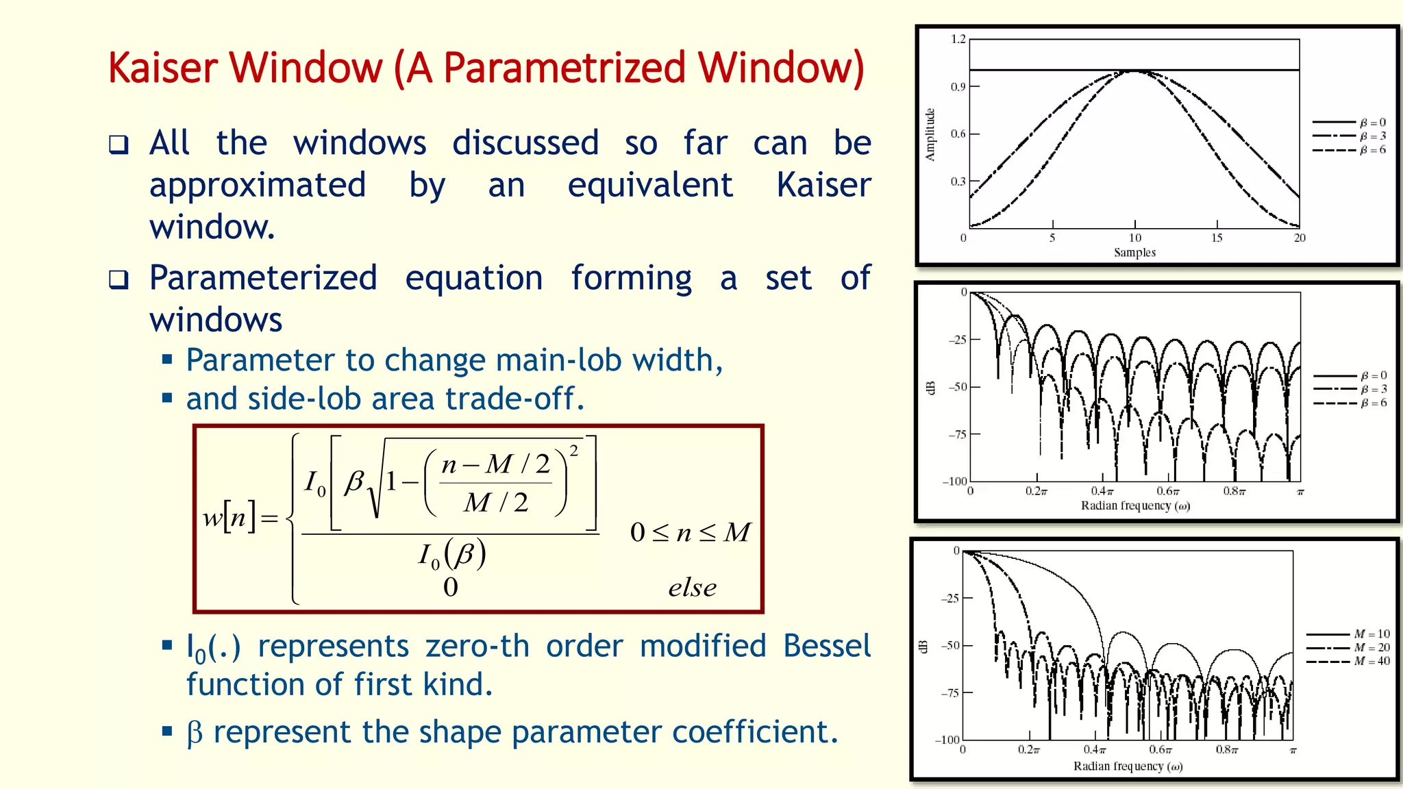
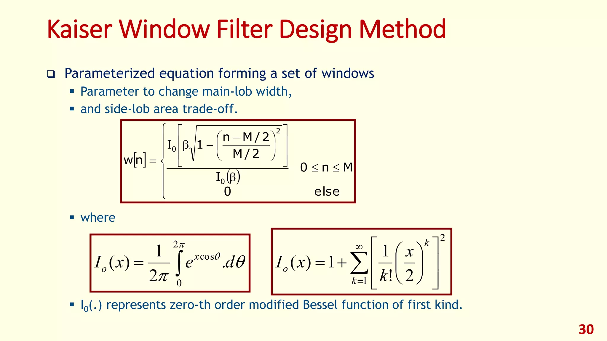
Kaiser window method adapts to design needs via parameterized control of response characteristics.
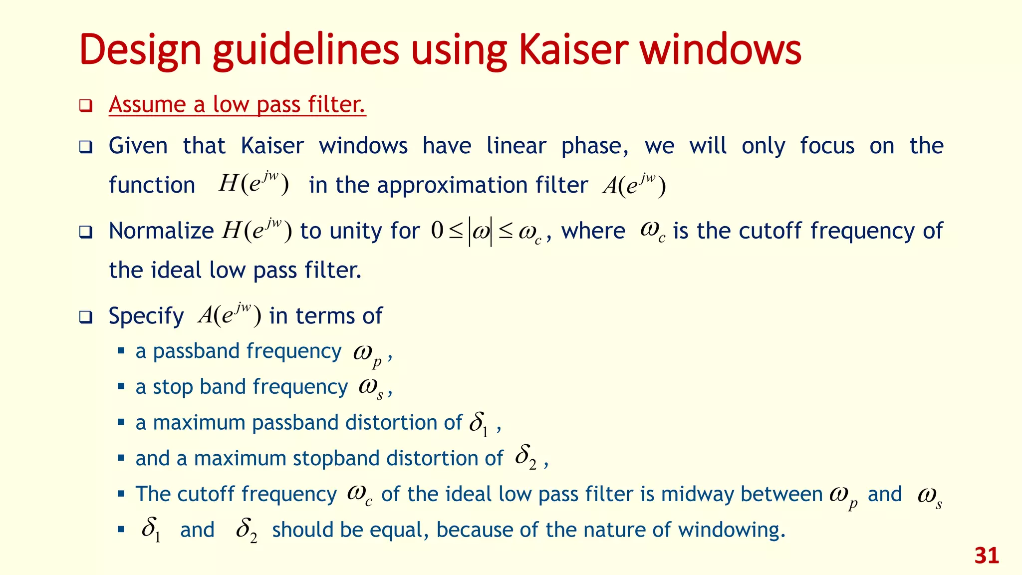
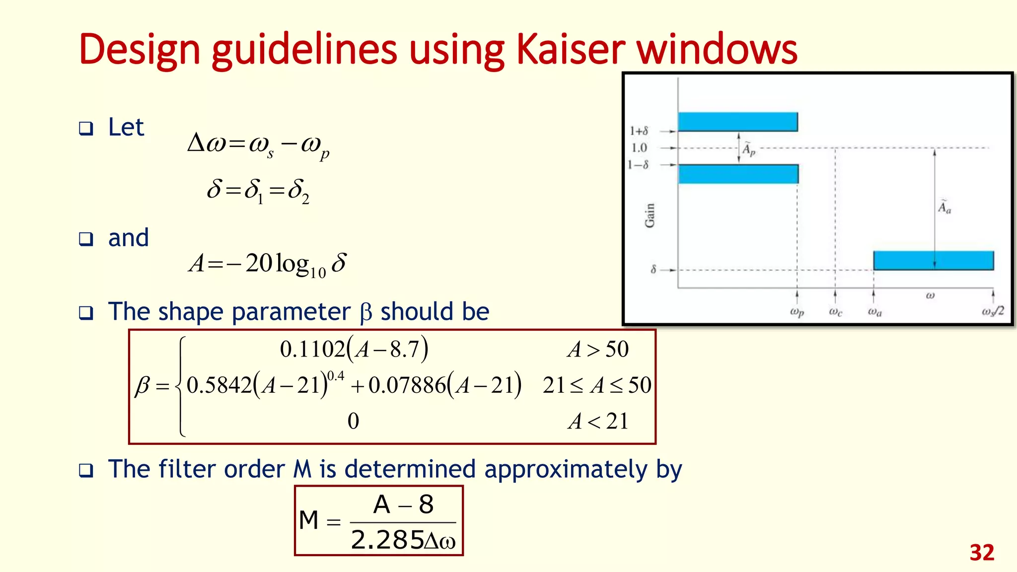
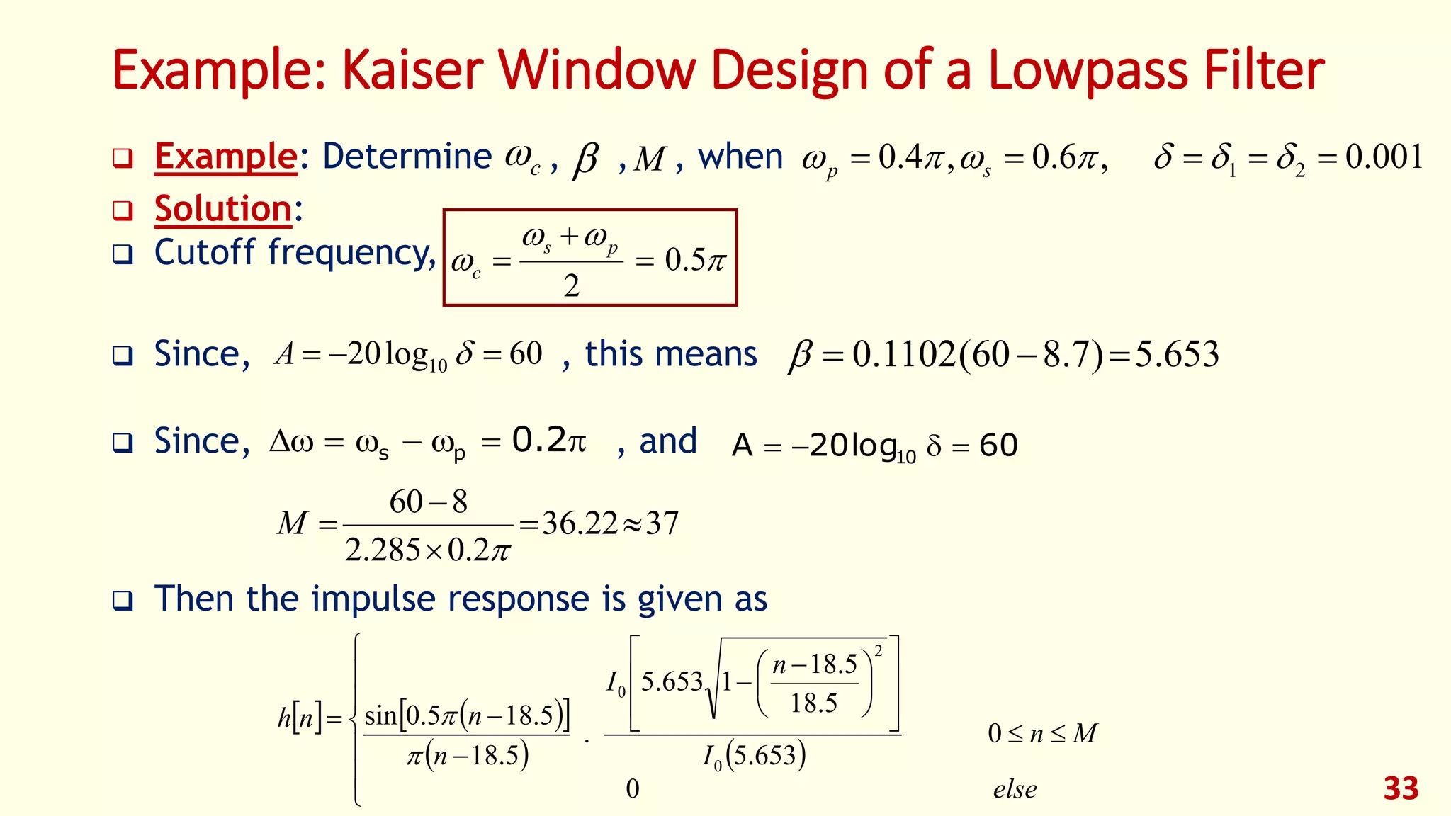
Designing with Kaiser windows involves setting passband/stopband parameters, calculating filter order.
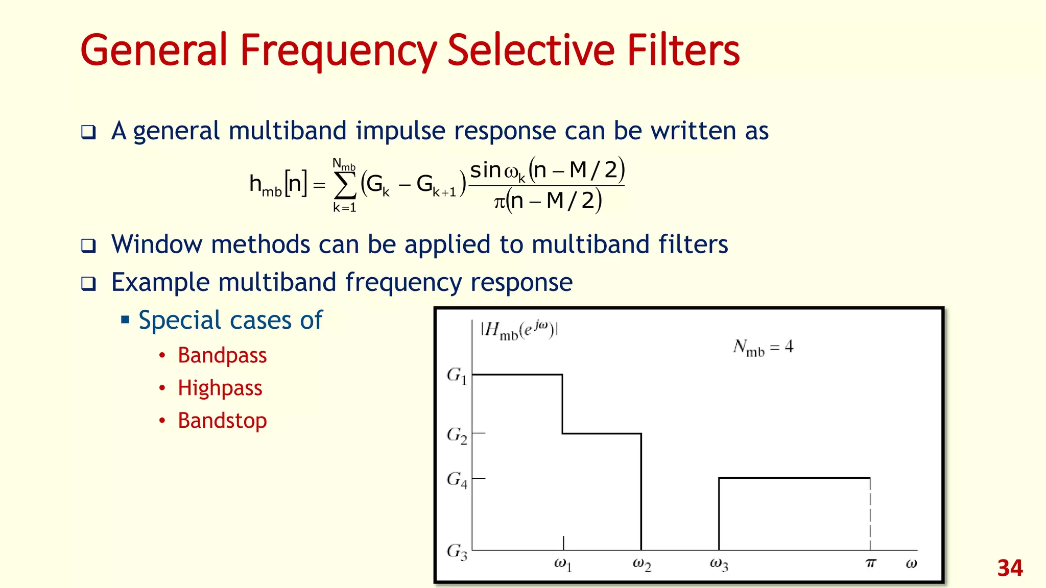
Application of windowing in multiband filter design and explanation of frequency sampling method challenges.