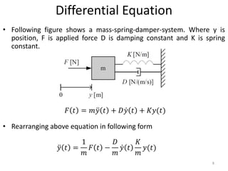
Downloaded 648 times
![Z-transform solution of Difference Equations
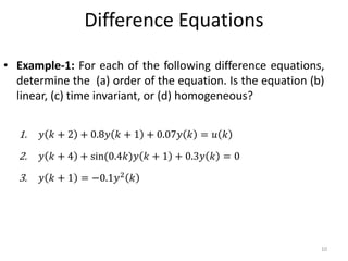
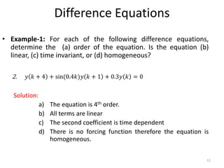
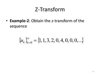
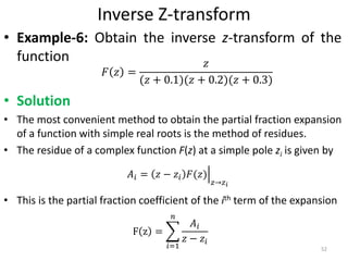
• Example-7: Solve the linear difference equation
• With initial conditions 𝑥 0 = 1, 𝑥 1 =
5
2
• 1. Taking z-transform of given equation
• 2. Solve for X(z)
54
𝑥 𝑘 + 2 −
3
2
𝑥 𝑘 + 1 +
1
2
𝑥 𝑘 = 1(𝑘)
Solution
𝑧2
𝑋 𝑧 − 𝑧2
𝑥 0 − 𝑧𝑥 1 −
3
2
𝑧𝑋 𝑧 +
1
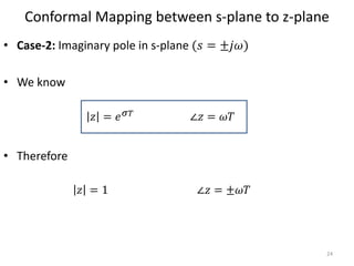
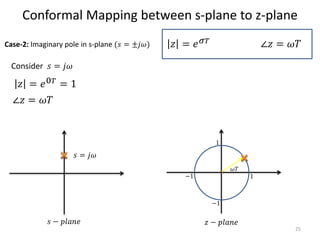
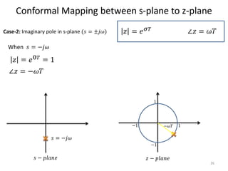
2
𝑋 𝑧 =
𝑧
𝑧 − 1
[𝑧2
−
3
2
𝑧 +
1
2
]𝑋 𝑧 =
𝑧
𝑧 − 1
+ 𝑧2
+ (
5
2
−
3
2
)𝑧](https://image.slidesharecdn.com/digitalcontrolsystemsdcslecture-18-19-20-160429131253/85/Digital-control-systems-dcs-lecture-18-19-20-54-320.jpg)
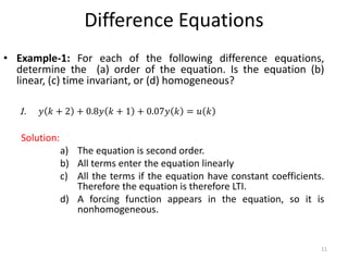
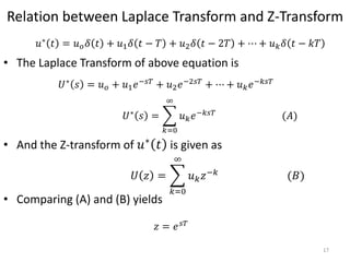
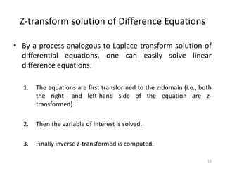
![Z-transform solution of Difference Equations
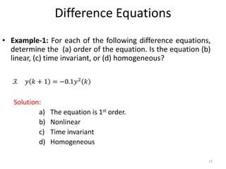
• Then
• 3. Inverse z-transform
55
[𝑧2
−
3
2
𝑧 +
1
2
]𝑋 𝑧 =
𝑧
𝑧 − 1
+ 𝑧2
+ (
5
2
−
3
2
)𝑧
𝑋 𝑧 =
𝑧[1 + (𝑧 + 1)(𝑧 − 1)]
(𝑧 − 1)(𝑧 − 1)(𝑧 − 0.5)
=
𝑧3
𝑧 − 1 2(𝑧 − 0.5)
𝑋 𝑧
𝑧
=
𝑧2
𝑧 − 1 2(𝑧 − 0.5)
=
𝐴
𝑧 − 1 2 +
𝐵
𝑧 − 1
+
𝐶
𝑧 − 0.5
𝑋(𝑧) =
2𝑧
𝑧 − 1 2
+
𝑧
𝑧 − 0.5
𝑥(𝑘) = 2𝑘 + (0.5) 𝑘](https://image.slidesharecdn.com/digitalcontrolsystemsdcslecture-18-19-20-160429131253/85/Digital-control-systems-dcs-lecture-18-19-20-55-320.jpg)

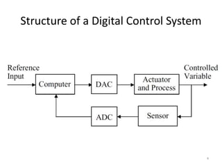
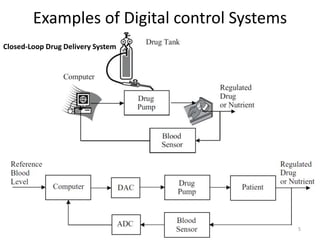
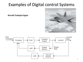
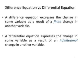
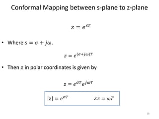
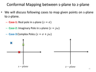
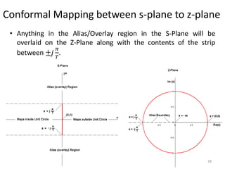
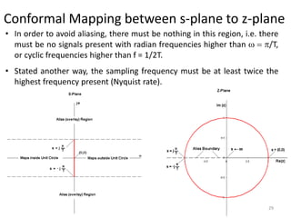
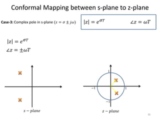
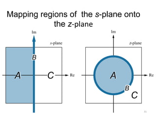
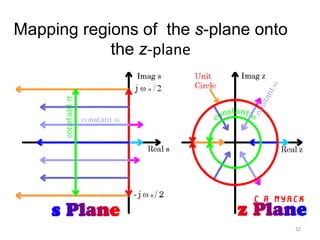
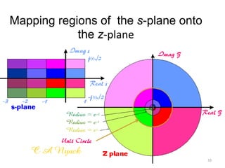
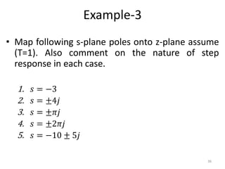
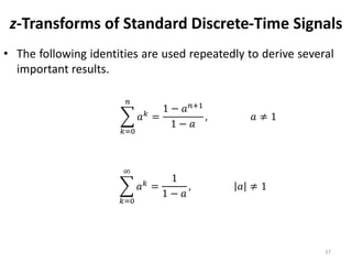
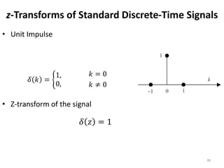
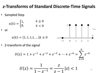
This document discusses digital control systems and related topics such as difference equations, z-transforms, and mapping between the s-plane and z-plane. It begins with an outline of topics to be covered including difference equations, z-transforms, inverse z-transforms, and the relationship between the s-plane and z-plane. Examples are provided to illustrate difference equations, z-transforms, and mapping poles between the two planes. Standard z-transforms of discrete-time signals like the unit impulse and sampled step are also defined.


