Downloaded 127 times


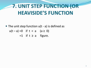
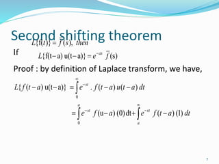
![Example: find the laplace
transform of t2 u(t-2)
solution:
L[f(t) u(t-a)]= e-as L[f(t+a)]
L [t2 u(t-2)] = e-2s L [(t+2)2 ]
= e-2s L [t2 + 4t+4]
= e-2s ( 2/s3 + 4/s2 + 4/s)](https://image.slidesharecdn.com/laplacesaahil-160917013100/85/Laplace-transform-UNIT-STEP-FUNCTION-SECOND-SHIFTING-THEOREM-DIRAC-DELTA-FUNCTION-6-320.jpg)
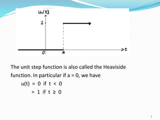
![( )
0
0
1
(u )) ,
(r)
(r) ( )
{ ( ) u(t a)} ( ) [ ( )]
[ ( )] ( ) ( )
st
a
s a r
as sr as
as as
as
e f a dt Substituting t a r
e f dr
e e f dr e f s
L f t a e f s e L f t
L e f s f t a u t a
8](https://image.slidesharecdn.com/laplacesaahil-160917013100/85/Laplace-transform-UNIT-STEP-FUNCTION-SECOND-SHIFTING-THEOREM-DIRAC-DELTA-FUNCTION-8-320.jpg)
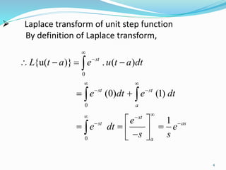
![.1: { ( ) ( )} [ ( )]
.2: [ ( )] [1. ( )] (1)
.3: [ ( ) ( )]
.4: [ ( ) { ( ) ( )] { ( )} { ( )}
as
as
as
as bs
as bs
Cor L f t u t a e L f t a
e
Cor L u t a L u t a e L
s
e e
Cor L u t a u t b
s
Cor L f t u t a u t b e L f t a e L f t b
(alternative form of second shifting theorem)
9](https://image.slidesharecdn.com/laplacesaahil-160917013100/85/Laplace-transform-UNIT-STEP-FUNCTION-SECOND-SHIFTING-THEOREM-DIRAC-DELTA-FUNCTION-9-320.jpg)

The document discusses the unit step function (also called the Heaviside function) and provides its definition and Laplace transform. It also discusses properties related to the Laplace transform of the unit step function, including: 1) The Laplace transform of the unit step function u(t-a) is 1/s when t ≥ a and 0 when t < a. 2) Using the shifting property, the Laplace transform of f(t)u(t-a) is e-asL[f(t+a)], where L[f(t)] is the Laplace transform of f(t). 3) An example calculates the Laplace transform of t2u(t-2) using the


