Download to read offline
![6
)
(
)
(
)
( s
E
s
G
s
Y
)
(
)
(
)
(
)
( s
Y
s
H
s
R
s
E
)
(
)
(
)
(
)
(
)
(
)]
(
)
(
)
(
)[
(
)
( s
Y
s
H
s
G
s
R
s
G
s
Y
s
H
s
R
s
G
s
Y
)
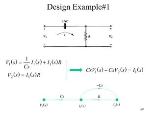
(
)
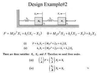
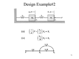
(
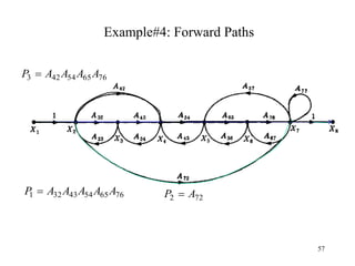
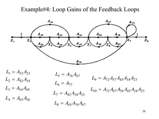
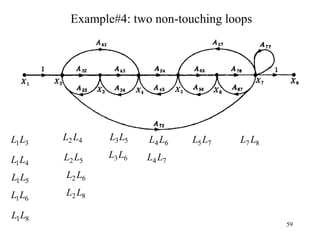
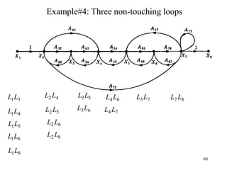
1
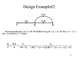
)
(
)
(
)
(
)
(
s
H
s
G
s
G
s
R
s
Y
s
T
](https://image.slidesharecdn.com/controlsystems-240529034436-780e8daa/85/block-diagram-and-signal-flow-graph-representation-6-320.jpg)
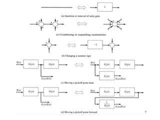
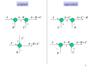
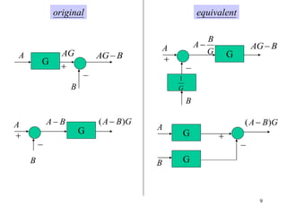
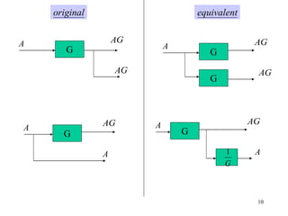
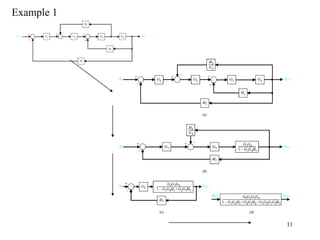
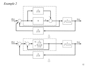
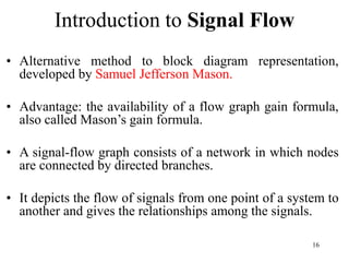
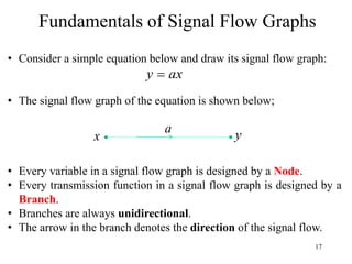
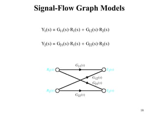
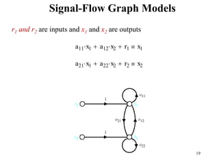
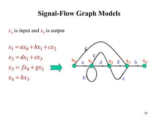
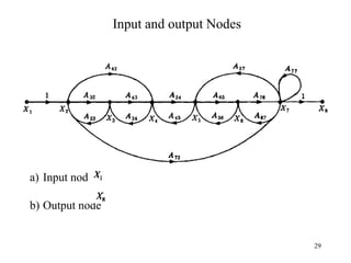
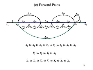
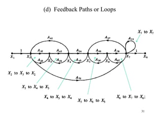
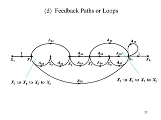
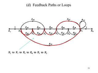
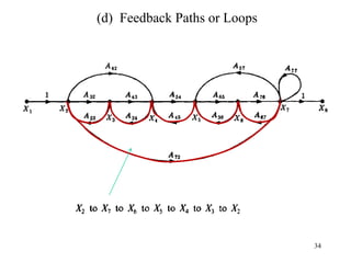
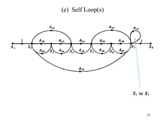
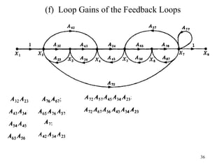
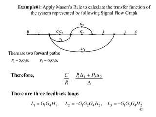
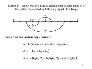
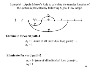
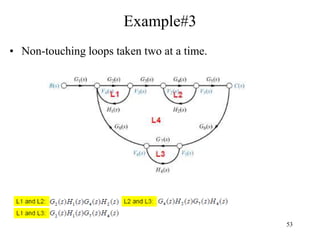
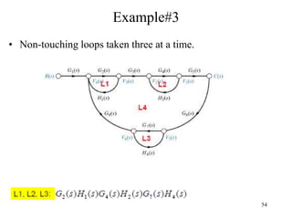
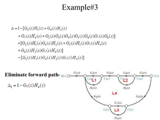
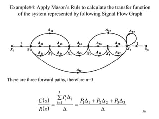

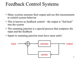
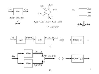
The document introduces block diagrams and signal flow graphs as tools for representing control systems, emphasizing their components and relationships. It explains feedback control systems where output is used to influence behavior, details signal flow graph terminology, and outlines Mason's rule for calculating transfer functions. Various examples illustrate the application of these concepts in analyzing and simplifying control engineering systems.


![Reduction of multiple subsystem [compatibility mode]](https://cdn.slidesharecdn.com/ss_thumbnails/reductionofmultiplesubsystemcompatibilitymode-110418075355-phpapp01-thumbnail.jpg?width=640&height=640&fit=bounds)


