This document discusses various properties and concepts related to the z-transform, which is used to analyze discrete-time signals. It defines the z-transform and region of convergence. It then provides examples of calculating the z-transform for different signals. Key properties discussed include time shifting, scaling, time reversal, differentiation, and convolution. Theorems regarding the initial value and final value are also covered. Worked examples are provided to demonstrate applying the various properties and concepts.

1. 1
Lecture 7 – 10
Z - Transform
June 07, 2005
By
Dr. Mukhtiar Ali Unar

2. 2
The Direct Z-Transform
The z-transform of a discrete time signal is defined as the power
series
(1)
Where z is a complex variable. For convenience, the z-transform of a
signal x[n] is denoted by
X(z) = Z{x[n]}
Since the z-transform is an infinite series, it exists only for those
values of z for which this series converges. The Region of
Convergence (ROC) of X(z) is the set of all values of z for which
this series converges.
We illustrate the concepts by some simple examples.






n
n
z
]
n
[
x
)
z
(
X

3. 3
Example 1: Determine the z-transform of
the following signals
(a) x[n] = [1, 2, 5, 7, 0, 1]
Solution: X(z) = 1 + 2z-1+ 5z-2 + 7z-3 + z-5,
ROC: entire z plane except z = 0
(b) y[n] = [1, 2, 5, 7, 0, 1]
Solution: Y(z) = z2 + 2z + 5 + 7z-1 + z-3
ROC: entire z-plane except z = 0 and z = .
(c) z[n] = [0, 0, 1, 2, 5, 7, 0, 1]
Solution: z-2 + 2z-3 + 5z-4 + 7z-5 + z-7, ROC: all z except z=0

4. 4
(d) p[n] = [n]
Solution: P(z) = 1, ROC: entire z-plane.
(e) q[n] = [n – k], k > 0
Solution: Q(z) = z-k, entire z-plane except
z=0.
(f) r[n] = [n+k], k > 0
Solution: R(z) = zk,
ROC: entire z-plane except z = .

5. 5
Example 2: Determine the z-transform of
x[n] = (1/2)nu[n]
Solution:
ROC: |1/2 z-1| < 1, or equivalently |z| > 1/2
1
2
1
n
0
n
1
n
n
0
n
n
n
z
2
1
1
1
.......
z
2
1
z
2
1
1
z
2
1
z
2
1
z
]
n
[
x
)
z
(
X












































6. 6
Example 3: Determine the z-transform of the
signal x[n] = anu[n]
Solution:
 
 
|
a
|
|
z
:|
ROC
az
1
1
.......
az
az
1
az
z
a
)
z
(
X
1
2
1
1
n
0
n
1
n
0
n
n





















7. 7
Properties of z-transform
 Linearity
If x1[n]  X1(z)
and x2[[n]  X2(z)
then
a1x1[n] + a2x2[n]  a1X1(z) + a2X2(z)

8. 8
Example: Determine the z-transform of
the signal x[n] = [3(2n) – 4(3n)]u[n]
Solution:
  1
1
n
n
1
n
z
3
1
1
4
z
2
1
1
3
]
3
4
)
2
(
3
[
z
az
1
1
]]
n
[
u
a
[
z












Example 4: Determine the z-transform of
the signal (cosw0n)u[n]
 
 
 
2
0
1
0
1
1
jw
1
jw
0
n
jw
n
jw
0
z
w
cos
z
2
1
w
cos
z
1
z
e
1
1
2
1
z
e
1
1
2
1
]
n
[
u
n
w
cos
z
e
2
1
e
2
1
]
n
[
u
n
w
cos
0
0
0
0




















9. 9
Time Shifting Property:
If x[n]  X(z) then x[n-k]  z-kX(z)
Proof:
since
then the change of variable m = n-k
produces








n
n
z
]
k
n
[
x
]]
k
n
[
x
[
z
)
z
(
X
z
z
]
m
[
x
z
z
]
m
[
x
]]
k
n
[
x
[
z
k
m
m
k
m
)
k
m
(


















10. 10
Example: Find the z-transform of a unit step
function. Use time shifting property to find z-
transform of u[n] – u[n-N].
The z-transform of u[n] can be found as
Now the z-transform of u[n]-u[n-N] may be
found as follows:
1
2
1
0
n
n
n
n
z
1
1
.......
z
z
1
z
z
]
n
[
u
]]
n
[
u
[
z

















 

1
N
1
N
1
z
1
z
1
z
1
1
z
z
1
1
]]
N
n
[
u
]
n
[
u
[
z















11. 11
Scaling in the z-domain
If x[n]  X(z)
Then anx[n]  X(a-1z)
For any constant a, real or complex.
Proof:
Example 5: Determine the z-transform of the signal
an(cosw0n)u[n].
Solution: since
     
z
a
X
z
a
]
n
[
x
z
]
n
[
x
a
]
n
[
x
a
z 1
n
n
1
n
n
n
n 











 

2
0
1
0
1
0
z
w
cos
z
2
1
w
cos
z
1
]
n
[
u
)
n
w
[cos(
z 






  2
2
0
1
0
1
0
n
z
a
w
cos
az
2
1
w
cos
az
1
]]
n
[
u
n
w
cos
a
[
z 








12. 12
Time reversal
If x[n]  X(z) then x[-n]  X(z-1)
Proof:
Example 6: Determine the z-transform of
u[-n].
Solution: since z[u[n]] = 1/(1 – z-1)
Therefore,
Z[u[-n]] = 1/(1-z)
 
 




















m m
1
m
1
m
n
n
)
z
(
X
z
]
m
[
x
z
]
m
[
x
z
]
n
[
x
]]
n
[
x
[
z

13. 13
Differentiation in the z - Domain
x[n]  X(z) then nx[n] = -z(dX(z)/dz)
Tutorial 4: Q1: Prove the differentiation
property of z – transform.
Example 7: Determine the z-transform of the
signal x[n] = nanu[n].
Solution:
 2
1
1
1
n
1
n
az
1
az
az
1
1
dz
d
z
]]
n
[
u
na
[
z
az
1
1
]]
n
[
u
a
[
z














14. 14
Convolution of two sequences
If x1[n]  X1(z) and x2[n]  X2(z) then
x1[n]*x2[n]  X1(z)X2(z)
Proof:
The convolution of x1[n] and x2[n] is defined as







k
2
1
2
1 ]
k
n
[
x
]
n
[
x
]
n
[
x
*
]
n
[
x
]
n
[
x
The z-transform of x[n] is
 
 





















n
n
n
2
1
n
n
z
k
n
x
]
k
[
x
z
]
n
[
x
)
z
(
X
Upon interchanging the order of the summation
and applying the time shifting property, we obtain
         
z
X
z
X
z
]
k
[
x
z
X
z
k
n
x
k
x
)
z
(
X 1
k
2
k
1
2
n
n
2
k
1 
























15. 15
Example 8: Compute the convolution
of the signals x1[n] = [1, -2, 1] and
Solution:
X1(z) = 1 – 2z-1 + z-2
X2(z) = 1 + z-1 + z-2 + z-3 + z-4 + z-5
Now X(z) = X1(z)X2(z) = 1 – z-1 – z-6 + z-7
Hence x[n] = [1, -1, 0, 0, 0, 0, -1, 1]
Note: You should verify this result from the
definition of the convolution sum.


 


elsewhere
,
0
5
n
0
,
1
]
n
[
x2

16. 16
Correlation of two sequences
If x1[n]  X1(z) and x2[n]  X2(z)
then rx1x2[k] = X1(z)X2(z-1)
 Tutorial 4 Q2: Prove this property.
The Initial Value Theorem:
If x[n] is causal then )
z
(
X
lim
]
0
[
x
z 


Proof:
....
z
]
2
[
x
z
]
1
[
x
]
0
[
x
z
]
n
[
x
)
z
(
X 2
1
0
n
n




 





Obviously, as z  , z-n  0 since n >0, this
proves the theorem.

17. 17
Final Value Theorem
If x[n]  X(z), then   )
z
(
X
z
1
lim
]
[
x 1
1
z





 Tutorial 4 Q3: Prove the Final Value
Theorem
Example 9: Find the final value of
2
1
1
z
8
.
0
z
8
.
1
1
z
2
)
z
(
X 





Solution:     2
1
1
1
1
z
8
.
0
z
8
.
1
1
z
2
z
1
)
z
(
X
z
1 









    1
1
1
1
1
1
z
5
.
0
1
z
2
z
5
.
0
1
z
1
z
2
z
1 











The final value theorem yields
10
2
.
0
2
z
8
.
0
1
z
2
lim
]
[
y 1
1
1
z




 



18. 18
Inverse z-transform
In general, the inverse z-transform may be
found by using any of the following
methods:
 Power series method
 Partial fraction method

19. 19
Power Series Method
Example 2: Determine the z-transform of
2
1
z
5
.
0
z
5
.
1
1
1
)
z
(
X 




By dividing the numerator of X(z) by its
denominator, we obtain the power series
...
z
z
z
z
1
z
z
1
1 4
16
31
3
8
15
2
4
7
1
2
3
2
2
1
1
2
3














 x[n] = [1, 3/2, 7/2, 15/8, 31/16,…. ]

20. 20
Power Series Method
Example 2:Determine the z-transform of
2
1
1
z
z
2
2
z
4
)
z
(
X 






By dividing the numerator of X(z) by its
denominator, we obtain the power series
 x[n] = [2, 1.5, 0.5, 0.25, …..]

21. 21
Partial Fraction Method:
Example 1: Find the signal corresponding to
the z-transform
2
1
3
z
z
3
2
z
)
z
(
X 





Solution:
  
5
.
0
z
1
z
z
5
.
0
z
5
.
0
z
5
.
1
z
5
.
0
z
z
3
2
z
)
z
(
X 2
3
2
1
3








 


   5
.
0
z
4
1
z
1
z
1
z
3
5
.
0
z
1
z
z
5
.
0
z
)
z
(
X
2
2










5
.
0
z
z
)
4
(
1
z
z
z
1
3
)
z
(
X







or 1
1
1
z
5
.
0
1
1
4
z
1
1
z
3
)
z
(
X 








  ]
n
[
u
5
.
0
4
]
n
[
u
]
1
n
[
]
n
[
3
]
n
[
x
n









22. 22
Partial Fraction Method:
Example 2: Find the signal corresponding to the z-
transform
  2
1
1
z
2
.
0
1
z
2
.
0
1
1
)
z
(
Y





Solution:
  2
3
2
.
0
z
2
.
0
z
z
)
z
(
Y



    2
2
2
2
.
0
z
1
.
0
2
.
0
z
75
.
0
2
.
0
z
25
.
0
2
.
0
z
2
.
0
z
z
z
)
z
(
Y









 2
2
.
0
z
z
1
.
0
2
.
0
z
z
75
.
0
1
z
z
25
.
0
)
z
(
Y






 2
1
1
2
.
0
1
.
0
1
1
z
2
.
0
1
z
2
.
0
z
2
.
0
1
1
75
.
0
z
2
.
0
1
1
25
.
0










      ]
n
[
u
2
.
0
n
5
.
0
]
n
[
u
2
.
0
75
.
0
]
n
[
u
2
.
0
25
.
0
]
n
[
y
n
n
n






23. 23
The One-Sided z-Transform
The one-sided or unilateral z-transform of a signal
x[n] is defined by





0
n
n
z
]
n
[
x
)
z
(
X
Characteristics:
•It does not contain information about the
signal x[n] for negative values of time.
• It is unique only for causal signals.

24. 24
Pulse Transfer Function
It is defined as the ratio of the z-transform of the
output to the z-transform of the input when all
initial conditions are assumed to be zero.
Mathematically,





















 N
0
k
k
k
M
0
k
k
k
N
N
2
2
1
1
0
M
M
2
2
1
1
0
z
a
z
b
z
a
.....
z
a
z
a
a
z
b
.....
z
b
z
b
b
)
z
(
H
The roots of the denominator of a pulse transfer function
are called Poles and those of the denominator are called
Zeros.
The above pulse transfer function has M zeros and N poles.
We can represent X(z) graphically by a pole-zero plot in the
Complex plane, which shows the location of poles by crosses
() and the location of zeros by circles (o).

25. 25
Stability:
A discrete time system is said to be stable if,
and only if, all of its poles lie inside a unit
circle.
If any pole(s) lie(s) on the unit circle, the
system is said to be marginally stable.
Im(z)
Re(z)




Unit circle
Stable System


Unstable System

Marginally stable

26. 26
Example: A system is characterized by
by the difference equation
y[n] – 0.1y[n-1] – 0.02 y[n-2] = 2x[n] – x[n-1].
Find the system transfer function and unit
impulse response.
Solution: Taking the z-transform of both sides of the
difference equation (ignoring the initial
conditions) we have
Y(z) – 0.1 z-1Y(z) – 0.02z-2Y(z) = 2X(z) – z-1X(z)
Y(z) [ 1 –0.1z-1 – 0.02z-2 ]= X(z [2 – z-1]
2
1
1
z
02
.
0
z
1
.
0
1
z
2
)
z
(
X
)
z
(
Y







This transfer function has two poles (i.e. z = -0.1, 0.2) and
Two zeros at z =0, 0.5. This shows that the system is
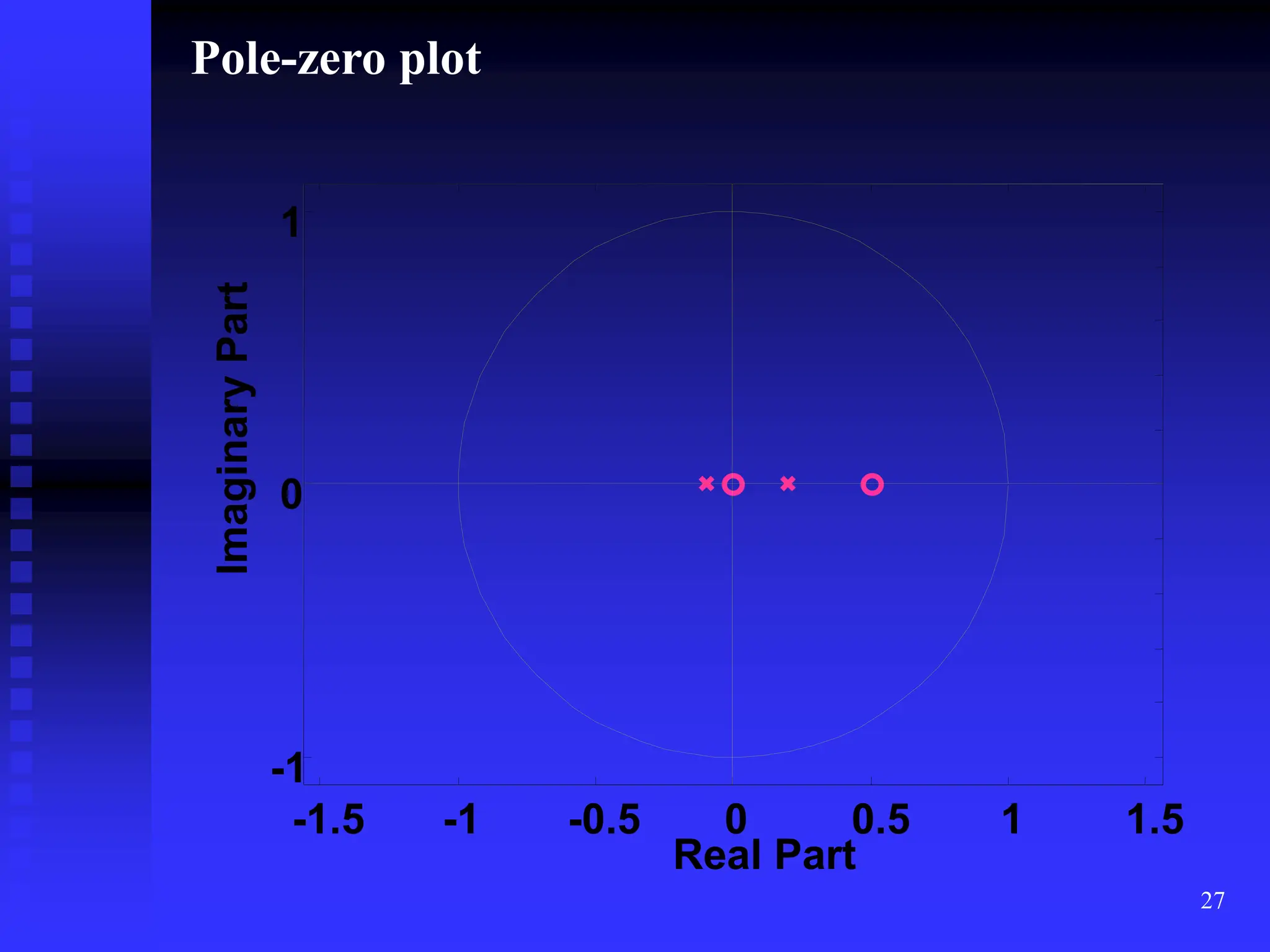
BIBO stable. The Pole-zero plot is given on the next slide.

27. 27
-1.5 -1 -0.5 0 0.5 1 1.5
-1
0
1
Real Part
Imaginary
Part
Pole-zero plot

28. 28
To find the unit impulse response, we
compute the inverse z-transform of H(z) by
using partial fraction expansion:
  
1
.
0
z
2
.
0
z
2
z
2
02
.
0
z
1
.
0
z
z
z
2
z
02
.
0
z
1
.
0
1
z
2
)
z
(
H
2
2
2
2
1
1











 


   1
.
0
z
4
2
.
0
z
2
1
.
0
z
2
.
0
z
1
z
2
z
)
z
(
H






























 
 1
1
z
1
.
0
1
1
4
z
2
.
0
1
1
2
1
.
0
z
z
4
2
.
0
z
z
2
)
z
(
H
and, the unit impulse response is
H[n] = -2(0.2)nu[n] + 4(-0.1)nu[n]

29. 29
Response of systems with non-zero initial
conditions
 We can use z-transform to solve the difference
equation that characterizes a causal, linear, time
invariant system. The following expressions are
especially useful to solve the difference
equations:
 z[y[(n-1)T] = z-1Y(z) +y[-T]
 Z[y(n-2)T] = z-2Y(z) + z-1y[-T] + y[-2T]
 Z[y(n-3)T] = z-3Y(z) + z-2y[-T] + z-1y[-2T] +
y[-3T]

30. 30
Tutorial 5 Q1: Determine the step response of
the system
y[n]=ay[n-1] + x[n], -1 < a < 1
when the initial condition is y[-1] = 1.

31. 31
Example: Consider the following difference
equation:
y[nT] –0.1y[(n-1)T] – 0.02y[(n-2)T] = 2x[nT] –
x[(n-1)T]
where the initial conditions are y[-T] = -10 and y[-
2T] = 20. Find the output y[nT] when x[nT] is the
unit step input.
Solution:
Computing the z-transform of the difference
equation gives
Y(z) – 0.1[z-1Y(z) + y[-T]] – 0.02[z-2Y(z) + z-1y[-T]
+ y[-2T]] = 2X(z) – z-1X(z)
Substituting the initial conditions we get
Y(z) – 0.1z-1Y(z) +1 – 0.02z-2Y(z) + 0.2z-1 –0.4 =
(2 – z-1)X(z)

32. 32
    6
.
0
z
2
.
0
z
1
1
z
2
)
z
(
Y
z
02
.
0
z
1
.
0
1 1
1
1
2
1






 




  6
.
0
z
2
.
0
z
1
z
2
z
02
.
0
z
2
.
0
1
)
z
(
Y 1
1
1
2
1






 




      
1
1
1
2
1
2
1
1
2
1
z
1
.
0
1
z
2
.
0
1
z
1
z
2
.
0
z
6
.
0
4
.
1
z
02
.
0
z
1
.
0
1
z
1
z
2
.
0
z
6
.
0
4
.
1
)
z
(
Y 





















   
1
.
0
z
2
.
0
z
1
z
z
2
.
0
z
6
.
0
z
4
.
1 2
3






1
.
0
z
830
.
0
2
.
0
z
567
.
0
1
z
136
.
1
z
)
z
(
Y







1
1
1
z
1
.
0
1
1
830
.
0
z
2
.
0
1
1
567
.
0
z
1
1
136
.
1
)
z
(
Y 








and the output signal y[nT] is
]
nT
[
u
)
1
.
0
(
830
.
0
]
nT
[
u
)
2
.
0
(
567
.
0
]
nT
[
u
136
.
1
]
nT
[
y n
n





33. 33
Pole-Zero Cancellation
 When a z-transform has a pole that is at the
same location as a zero, the pole is cancelled by
the zero and, consequently, the term containing
that pole in the inverse z-transform vanishes.
 Pole-zero cancellation may occur either in the
system function itself or in the product of the
system function with the z-transform of the
input signal.
 When the zero is located very near the pole but
not exactly at the same location, the term in the
response has a very small amplitude.
 Pole-zero cancellation may cause instability
and should be avoided in most cases.

34. 34
Example: Determine the unit impulse response of
the system characterized by the difference
equation
y[n] = 2.5y[n-1] – y[n-2] + x[n] – 5x[n-1] + 6x[n-2]
Solution: Taking the z-transform of both sides of
the above difference equation and ignoring all
initial conditions, we obtain the following pulse
transfer function:
  
   1
2
1
1
1
2
1
1
1
1
2
1
1
1
2
1
2
1
z
1
z
5
.
2
1
z
1
z
3
1
z
2
1
z
1
z
3
1
z
2
1
z
z
5
.
2
1
z
6
z
5
1
)
z
(
H 



























and therefore
  ]
1
n
[
u
5
.
2
]
n
[
]
n
[
h
1
n
2
1






35. 35
System Frequency response
The frequency response of a BIBO stable
system is defined as
H(w) = H(z)|z = e
jw
The frequency response function is usually
expressed in terms of its magnitude |H(w)|
and phase (w), where
H(w) = |H(w)|ej(w)
Usually, the magnitude is plotted on a
logarithmic scale as
|H(w)|dB = 20log10|H(w)|

36. 36
Example: Determine the frequency response
function H(w) and the magnitude |H(w)|dB for the
LTI system characterized by the difference
equation
y[n] = 1.8y[n-1] – 0.81y[n-2] + x[n] + 0.95x[n-1]
Solution: The pulse transfer function is
 2
1
1
2
1
1
z
9
.
0
1
z
95
.
0
1
z
81
.
0
z
8
.
1
1
z
95
.
0
1
)
z
(
H












Now the frequency response function may be obtained as
 
 2
jw
jw
e
9
.
0
1
e
95
.
0
1
w
H





The magnitude response is
w
cos
8
.
1
81
.
1
w
cos
9
.
1
9025
.
1
|
)
w
(
H
|




37. 37
We note that |H(w)| has its maximum at w = 0,
where |H(0)| = 195. It is customary to normalize
|H(w)| by its peak value and plot
20log|H(w)|/|H|max. A plot of the normalized
magnitude of the frequency response is shown
below:
0
-90
-80
-70
-60
-50
-40
-30
-20
-10
0
- 

38. 38
Example: Find the frequency response for the
system
y[n] = -0.1y[n-1] + 0.2y[n-2] + x[n] + x[n-1]
Solution: The system function is
2
1
1
z
2
.
0
z
1
.
0
1
z
1
)
z
(
H 






Now
)
z
z
(
2
.
0
)
z
z
(
08
.
0
05
.
1
z
z
2
z
2
.
0
z
1
.
0
1
z
1
z
2
.
0
z
1
.
0
1
z
1
)
z
(
H
)
z
(
H 2
2
1
1
2
2
1
1
1





















w
cos
8
.
0
w
cos
16
.
0
45
.
1
w
cos
2
2
|
)
z
(
H
)
z
(
H
|
|
)
w
(
H
| 2
e
z
1
2
jw




 

w
cos
8
.
0
w
cos
16
.
0
45
.
1
w
cos
2
2
|
)
w
(
H
| 2




