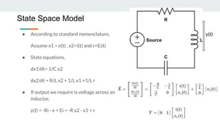
This presention is about one of the most important concept of control system called State space analysis. Here basic concept of control system and state space are discussed.
NONLINEAR CONTROL SYSTEM(Phase plane & Phase Trajectory Method)Niraj Solanki
This document discusses nonlinear control systems using phase plane and phase trajectory methods. It defines nonlinear systems and common physical nonlinearities like saturation, dead zone, relay, and backlash. Phase plane analysis is introduced as a graphical method to study nonlinear systems using a plane with state variables x and dx/dt. Key concepts are defined like phase plane, phase trajectory, and phase portrait. Methods for sketching phase trajectories include analytical solutions and graphical methods using isoclines. Examples are given to illustrate phase portraits for different linear systems.
This presentation explains about the introduction of Polar Plot, advantages and disadvantages of polar plot and also steps to draw polar plot. and also explains about how to draw polar plot with an examples. It also explains how to draw polar plot with numerous examples and stability analysis by using polar plot.
The document discusses time domain analysis and standard test signals used to analyze dynamic systems. It describes the impulse, step, ramp, and parabolic signals which imitate characteristics of actual inputs such as sudden shock, sudden change, constant velocity, and constant acceleration. The time response of first order systems to these standard inputs is expressed mathematically. The impulse response directly provides the system transfer function. Step response reaches 63% of its final value within one time constant.
State space analysis, eign values and eign vectorsShilpa Shukla
This document discusses state space analysis and the conversion of transfer functions to state space models. It covers:
1. The need to convert transfer functions to state space form in order to apply modern time domain techniques for system analysis and design.
2. Three possible representations for realizing a transfer function as a state space model: first companion form, second companion form, and Jordan canonical form.
3. The concepts of eigenvalues and eigenvectors, and how they relate to state space models.
4. Worked examples of converting transfer functions to state space models in first and second companion forms, as well as the Jordan canonical form for systems with repeated and non-repeated roots.
The document provides an overview
Digital controllers have several advantages over analog controllers, including flexibility, decision-making capability, and high performance for a lower cost. They can also be easily designed and tested through simulations. A digital control system uses analog to digital converters to digitize sensor signals and digital to analog converters to generate control signals. It samples continuous sensor signals and holds the values constant between samples, introducing quantization error that can be reduced by increasing the number of quantization levels.
This document discusses discrete-time signals and sequences. It defines discrete-time signals as sequences of numbers represented as x[n], where n is an integer. In practice, sequences arise from periodically sampling an analog signal. Linear time-invariant (LTI) systems are described by the convolution sum, where the impulse response h[n] completely characterizes the system. FIR systems have impulse responses of finite duration, while IIR systems can have impulse responses that extend to infinity.
The document discusses the concepts of controllability and observability in state space analysis of dynamic systems. It defines controllability as the ability to transfer a system state to any desired state using control inputs. Observability is defined as the ability to identify the system state using output measurements. Gilbert's and Kalman's tests are described to check for complete controllability and observability by examining the system and output matrices. No cancellation of poles and zeros in the transfer function is a necessary condition for complete controllability and observability.
This paper outlines fundamental topics related to classical control theory. It moves from modeling simple mechanical systems to designing controllers to manage said system.
This chapter discusses digital control systems. It describes the components of a digital control loop including digital controllers, analog-to-digital converters (ADCs), and digital-to-analog converters (DACs). ADCs convert analog signals to digital words, while DACs convert digital words to analog signals. Proper sampling and holding is required for interfacing between analog and digital systems. The sampling frequency must be high enough to avoid aliasing, with a recommended rate of 6-25 times the bandwidth of the controlled process.
This Presentation explains about the introduction of Frequency Response Analysis. This video clearly shows advantages and disadvantages of Frequency Response Analysis and also explains frequency domain specifications and derivations of Resonant Peak, Resonant Frequency and Bandwidth.
This document discusses and compares the classical/transfer function approach and the state space/modern control approach for modeling dynamical systems. The classical approach uses Laplace transforms and transfer functions in the frequency domain, while the state space approach uses matrices to represent systems of differential equations directly in the time domain. The state space approach can model nonlinear, time-varying, and multi-input multi-output systems and considers initial conditions, while the classical approach is limited to linear time-invariant single-input single-output systems. The document provides examples of modeling circuits using the state space representation.
Dcs lec03 - z-analysis of discrete time control systemsAmr E. Mohamed
The document discusses discrete time control systems and their mathematical representation using z-transforms. It covers topics such as impulse sampling, the convolution integral method for obtaining the z-transform, properties of the z-transform, inverse z-transforms using long division and partial fractions, and mapping between the s-plane and z-plane. Examples are provided to illustrate various concepts around discrete time systems and their analysis using z-transforms.
The document provides an overview of digital control systems, including the sampling process and Z-transform. It defines digital and analog signals, and explains how data acquisition works by sampling analog signals and converting them to digital values using analog-to-digital converters. Examples are given of number systems, signal conditioning, and the sampling process theory. Matlab samples are also provided to demonstrate continuous and discrete signals.
Modern Control - Lec07 - State Space Modeling of LTI SystemsAmr E. Mohamed
The document provides an overview of state-space representation of linear time-invariant (LTI) systems. It defines key concepts such as state variables, state vector, state equations, and output equations. Examples are given to show how to derive the state-space models from differential equations describing dynamical systems. Specifically, it shows how to 1) select state variables, 2) write first-order differential equations as state equations, and 3) obtain output equations to fully represent LTI systems in state-space form.
The document discusses the z-transform, which is a mathematical tool used to analyze discrete-time control systems. The z-transform plays a similar role for discrete-time systems as the Laplace transform does for continuous-time systems. Some key properties of the z-transform discussed include the region of convergence, properties and theorems like the shifting theorem and initial/final value theorems, and applications to feedback control systems.
Chapter 7 Controls Systems Analysis and Design by the frequency response analysis . From the book (Ogata Modern Control Engineering 5th).
7-1 introduction.
7-2 Bode diagrams.
This document provides an overview of transfer functions and stability analysis of linear time-invariant (LTI) systems. It discusses how the Laplace transform can be used to represent signals as algebraic functions and calculate transfer functions as the ratio of the Laplace transforms of the output and input. Poles and zeros are introduced as important factors for stability. A system is stable if all its poles reside in the left half of the s-plane and unstable if any pole resides in the right half-plane. Examples are provided to demonstrate calculating transfer functions from differential equations and analyzing stability based on pole locations.
ppt on Time Domain and Frequency Domain Analysissagar_kamble
in this presentation, you will be able to know what is this freq. and time domain analysis.
At last one example is illustreted with video, which distinguishes these two analysis
Digital control systems (dcs) lecture 18-19-20Ali Rind
This document discusses digital control systems and related topics such as difference equations, z-transforms, and mapping between the s-plane and z-plane. It begins with an outline of topics to be covered including difference equations, z-transforms, inverse z-transforms, and the relationship between the s-plane and z-plane. Examples are provided to illustrate difference equations, z-transforms, and mapping poles between the two planes. Standard z-transforms of discrete-time signals like the unit impulse and sampled step are also defined.
Modern Control - Lec 02 - Mathematical Modeling of SystemsAmr E. Mohamed
This document provides an overview of mathematical modeling of physical systems. It discusses how to derive mathematical models from physical systems using differential equations based on governing physical laws. The key steps are: (1) defining the physical system, (2) formulating the mathematical model using differential equations, and (3) solving the equations. Common model types include differential equation, transfer function, and state-space models. The document also discusses modeling various physical elements like electrical circuits, mechanical translational/rotational systems, and electro-mechanical systems using differential equations. It covers block diagram representation and reduction of mathematical models. The overall goal is to realize the importance of deriving accurate mathematical models for analyzing and designing control systems.
This document discusses deadbeat response design for digital control systems. It covers:
1. Designing controllers to achieve a deadbeat response when plant poles and zeros are inside the unit circle. The controller must cancel plant poles to achieve zero steady state error within a finite number of samples.
2. Examples where the controller achieves a deadbeat response of 1 sample for a step input and 2 samples for a ramp input.
3. Considerations for designing deadbeat responses when some plant poles and zeros are on or outside the unit circle, where imperfect cancellation could lead to instability. The controller must not cancel these poles and zeros.
4. Achieving a deadbeat response in sampled data control systems without
Transmission lines are physical connections between two locations that transmit electromagnetic waves. They have characteristic parameters including resistance, inductance, capacitance, and conductance per unit length. These parameters depend on the line's geometry and materials. Transmission line equations relate the voltage and current at each point on the line based on these parameters. A line has a characteristic impedance that is the ratio of voltage to current. Reflection and transmission of waves occurs at impedance discontinuities like at the load. Lossless lines propagate waves without attenuation, while finite lines are analyzed using reflection coefficients at the generator and load terminations.
Time response of discrete systems 4th lecturekhalaf Gaeid
1. The document discusses the time response of discrete-time systems, including their transient and steady-state response. It describes parameters for characterizing transient response such as rise time, delay time, peak time, and settling time.
2. Steady-state errors are also examined for different system types (Type-0, 1, 2 systems) and inputs (step, ramp, parabolic). Examples are provided to calculate steady-state errors.
3. The response of discrete-time systems is derived using impulse response sequences and convolution sums. The time response is broken into zero-input and zero-state responses.
Ch5 transient and steady state response analyses(control)Elaf A.Saeed
Chapter 5 Transient and steady-state response analyses. From the book (Ogata Modern Control Engineering 5th).
5-1 introduction.
5-2 First-Order System.
5-3 second-order system.
5-6 Routh’s stability criterion.
5-8 Steady-state errors in unity-feedback control systems.
This document discusses signals and their classification. It defines signals, analog and digital signals, periodic and aperiodic signals. It also discusses representing signals in Matlab and Simulink. Key signal types covered include exponential, sinusoidal, unit impulse and step functions. Matlab is presented as a tool for programming and analyzing discrete signals while Simulink can be used to model and simulate continuous systems.
First & second order of the control systemsSatheeshCS2
This document summarizes key concepts about first and second order control systems. It discusses:
- The characteristics of a first order system, which has one pole and is defined by its DC gain (K) and time constant (T).
- Examples of first order systems and how to determine their DC gain and time constant.
- That a second order system can have different responses depending on its parameters, such as damped or undamped oscillations.
- How to determine the undamped natural frequency and damping ratio of a second order system by comparing its transfer function to the general second order transfer function.
The document then provides example problems for determining properties of first and second order systems. It concludes by
The document discusses different types of singular points in control systems:
1. A nodal point occurs when both eigenvalues are real and negative, causing all trajectories to converge to the origin in a stable manner.
2. A saddle point occurs when the eigenvalues are real and equal but opposite in sign, making the origin unstable with some trajectories converging and others diverging.
3. A focus point occurs when the eigenvalues are complex conjugates with negative real parts, causing the trajectories to spiral inward in a stable manner towards the origin.
4. A center or vortex point occurs when the eigenvalues are purely imaginary, causing the trajectories to travel in closed paths around the origin in a limitedly stable manner.
PPTS on Topic-PLC
In this ppts there is simple introduction to plc and one example of project using PLC. This also include programming for the given project (Metal segregation using PLC)
This document provides an introduction to state space modeling and analysis in modern control systems. It defines key concepts such as state, state variables, state vector, and state space. The document describes how to represent dynamic systems using state space equations involving state variables, input variables, output variables, and state vectors. It provides examples of modeling a mechanical system and DC motor in state space form. It also discusses the concept of state controllability and how to determine if a system is completely controllable using the controllability matrix.
This document discusses state space representation of systems. It begins by outlining how to find a state space model for a linear time-invariant system using state equations and matrices. It then provides examples of deriving state space models for electrical, mechanical, and electromechanical systems. The document also covers converting between transfer functions and state space models, and defines key terms like state vector, state space, controllability, and observability.
State-Space Analysis of Control System: Vector matrix representation of state equation, State transition matrix, Relationship between state equations and high-order differential equations, Relationship between state equations and transfer functions, Block diagram representation of state equations, Decomposition Transfer Function, Kalman’s Test for controllability and observability
State space analysis provides a powerful modern approach for modeling and analyzing control systems. It represents a system using state variables and state equations. This allows incorporating initial conditions, applying to nonlinear/time-varying systems, and providing insight into the internal state of the system. A state space model consists of state equations describing how the state variables change over time, and output equations relating the outputs to the states and inputs. Common applications include modeling physical dynamic systems using energy-storing elements as states, and obtaining linear models for linear time-invariant systems. State space analysis provides advantages over traditional transfer function methods.
Introduction to Hybrid Vehicle System Modeling and Control - 2013 - Liu - App...sravan66
This document discusses mathematical modeling of hybrid vehicle systems. It begins by explaining the two main approaches to building mathematical models: using physical principles or observed system behaviors. Dynamic systems can be modeled using differential equations, state space equations, or transfer functions. Models are classified as static/dynamic, time-varying/invariant, deterministic/stochastic, continuous/discrete, linear/nonlinear, and lumped-parameter/distributed-parameter. State space models represent systems using state vectors, input vectors, output vectors, and coefficient matrices to describe the relationships between these variables.
This document provides an overview of signals and systems. It defines a signal as a physical quantity that varies with time and contains information. Signals are classified as deterministic or non-deterministic, periodic or aperiodic, even or odd, energy-based or power-based, and continuous-time or discrete-time. Systems are combinations of elements that process input signals to produce output signals. Key properties of systems include causality, linearity, time-invariance, stability, and invertibility. Applications of signals and systems are found in control systems, communications, signal processing, and more.
This document provides an introduction to dynamical systems and their mathematical modeling using differential equations. It discusses modeling dynamical systems using inputs, states, and outputs. It also covers simulating dynamical systems, equilibria, linearization, and system interconnections. Key topics include modeling dynamical systems using differential equations, the concept of inputs and outputs, interpreting mathematical models of dynamical systems, and converting higher-order models to first-order models.
Sensors by computer applications gghhhhhhhhhhhhhhhhhhhhhhffffffffffffffffffffffffffffgffggttttsvbkihhhggttfffffffffffffffffggggttggggyyyyy h ilc you k fd7ihft I yft8iggd e u hbvd67ufr6uufffhjoytrdfhiigfffghj I cc c for judging Jukka c ffffg b gffryhhu.
Nn h Todd I k he kidd cnn I kgf um b dc m l1234567889pp2356789p002224564221356788
UNIT-V-PPT state space of system model .pptabbas miry
1. There are two main approaches for analyzing and designing control systems: the classical/frequency domain technique using transfer functions and the modern/time domain technique using state-space models.
2. State-space models represent a system using matrices and vectors of input, output, and state variables related by first-order differential equations. This allows analysis of systems with multiple inputs and outputs and knowledge of internal states.
3. A state-space model defines state variables that contain the minimum information needed to describe the system behavior. The state-space is an n-dimensional space with axes defined by the state variables.
The document discusses state variable models for analyzing physical systems described by differential equations. It introduces state variables as a set of variables that can be used to represent a system's dynamic behavior through first-order differential equations. These state differential equations can be written in matrix form and describe how the rate of change of the state variables is related to the state variables and input functions over time. The state variable approach allows for computer analysis and modeling of nonlinear, time-varying, and multivariable systems.
Julio Bravo's Master Graduation ProjectJulio Bravo
The document describes applying an optimal control tracking problem to a wind power system to track desired trajectories of system states. It presents the nonlinear mathematical model of a wind power system and linearizes it around operating points. It then formulates the optimal control problem to minimize errors from desired trajectories, subject to system dynamics. The solution provides control inputs to drive the system states to follow the desired trajectories over time.
The document provides information about state variable models and transfer functions. It discusses:
- Modeling systems using state variables and representing them with first-order differential equations in matrix form.
- Obtaining transfer functions from state variable models by taking the Laplace transform of the state equations.
- Examples of modeling an RLC circuit and calculating its transfer function from the state equations.
- Using state variable models and feedback to design state variable feedback control systems. This involves estimating unmeasured states with observers and connecting the observer to the full-state feedback control law.
The document provides an overview of state-space representation of linear time-invariant (LTI) systems. It defines the state of a dynamical system and explains that the state-space approach models systems using sets of first-order differential equations rather than transfer functions. The key advantages of the state-space approach include its ability to model more complex multi-input multi-output systems and incorporate internal system behavior. Examples are provided to demonstrate how higher-order systems can be converted to state-space form by defining state variables and writing the corresponding state equations.
This document discusses state space analysis and related concepts. It defines state as a group of variables that summarize a system's history to predict future outputs. The minimum number of state variables required is equal to the number of storage elements in the system. These state variables form a state vector. The document also covers state space representation, diagonalization, solving state equations, the state transition matrix, and concepts of controllability and observability.
This document discusses control systems and their analysis using state space models. It defines the key components of a control system and explains how state space representation models systems using state variables and matrices. The document also covers analyzing stability, controllability and observability of state space models.
- The document details a state space solver approach for analog mixed-signal simulations using SystemC. It models analog circuits as sets of linear differential equations and solves them using the Runge-Kutta method of numerical integration.
- Two examples are provided: a digital voltage regulator simulation and a digital phase locked loop simulation. Both analog circuits are modeled in state space and simulated alongside a digital design to verify mixed-signal behavior.
- The state space approach allows modeling analog circuits without transistor-level details, improving simulation speed over traditional mixed-mode simulations while still capturing system-level behavior.
This document discusses system modeling and properties of linearity and time invariance. It provides examples of modeling a resistor, square-law system, delay operator, and time compressor to illustrate these properties. A model is a set of mathematical equations relating the output and input signals of a physical system. A system is linear if the response to a sum of inputs is the sum of the responses. It is time invariant if its behavior does not change over time. Developing an accurate but simplified model is important for understanding system behavior and designing controllers.
1. The document discusses methods for calculating summary statistics for continuous-time Markov chains (CTMCs), which are used to model processes like DNA sequence evolution.
2. It focuses on calculating the expected number of jumps between states and expected waiting time in a state, conditioned on the start and end points. These statistics are needed to estimate model parameters using maximum likelihood approaches like the EM algorithm.
3. As an application, the document describes using a 61x61 CTMC rate matrix to model codon sequence evolution, with the matrix parameters estimated via the EM algorithm using the summary statistics. Expected jumps between states differentiated by transition type are of particular interest.
This document introduces linear time-varying (LTV) systems and the computation of the state transition matrix (STM) for LTV systems. It discusses:
1) The definition and properties of the STM for LTV systems.
2) Conditions under which the system matrix A(t) commutes with the integral of A(t), which is required to compute the STM.
3) Examples of computing the STM for different time-varying system matrices.
4) How to obtain the overall state solution for an LTV system given its STM.
5) An introduction to discretizing continuous-time systems.
state space representation,State Space Model Controllability and Observabilit...Waqas Afzal
State Variables of a Dynamical System
State Variable Equation
Why State space approach
Block Diagram Representation Of State Space Model
Controllability and Observability
Derive Transfer Function from State Space Equation
Time Response and State Transition Matrix
Eigen Value
Introduction- e - waste – definition - sources of e-waste– hazardous substances in e-waste - effects of e-waste on environment and human health- need for e-waste management– e-waste handling rules - waste minimization techniques for managing e-waste – recycling of e-waste - disposal treatment methods of e- waste – mechanism of extraction of precious metal from leaching solution-global Scenario of E-waste – E-waste in India- case studies.
ACEP Magazine edition 4th launched on 05.06.2024Rahul
This document provides information about the third edition of the magazine "Sthapatya" published by the Association of Civil Engineers (Practicing) Aurangabad. It includes messages from current and past presidents of ACEP, memories and photos from past ACEP events, information on life time achievement awards given by ACEP, and a technical article on concrete maintenance, repairs and strengthening. The document highlights activities of ACEP and provides a technical educational article for members.
Advanced control scheme of doubly fed induction generator for wind turbine us...IJECEIAES
This paper describes a speed control device for generating electrical energy on an electricity network based on the doubly fed induction generator (DFIG) used for wind power conversion systems. At first, a double-fed induction generator model was constructed. A control law is formulated to govern the flow of energy between the stator of a DFIG and the energy network using three types of controllers: proportional integral (PI), sliding mode controller (SMC) and second order sliding mode controller (SOSMC). Their different results in terms of power reference tracking, reaction to unexpected speed fluctuations, sensitivity to perturbations, and resilience against machine parameter alterations are compared. MATLAB/Simulink was used to conduct the simulations for the preceding study. Multiple simulations have shown very satisfying results, and the investigations demonstrate the efficacy and power-enhancing capabilities of the suggested control system.
Electric vehicle and photovoltaic advanced roles in enhancing the financial p...IJECEIAES
Climate change's impact on the planet forced the United Nations and governments to promote green energies and electric transportation. The deployments of photovoltaic (PV) and electric vehicle (EV) systems gained stronger momentum due to their numerous advantages over fossil fuel types. The advantages go beyond sustainability to reach financial support and stability. The work in this paper introduces the hybrid system between PV and EV to support industrial and commercial plants. This paper covers the theoretical framework of the proposed hybrid system including the required equation to complete the cost analysis when PV and EV are present. In addition, the proposed design diagram which sets the priorities and requirements of the system is presented. The proposed approach allows setup to advance their power stability, especially during power outages. The presented information supports researchers and plant owners to complete the necessary analysis while promoting the deployment of clean energy. The result of a case study that represents a dairy milk farmer supports the theoretical works and highlights its advanced benefits to existing plants. The short return on investment of the proposed approach supports the paper's novelty approach for the sustainable electrical system. In addition, the proposed system allows for an isolated power setup without the need for a transmission line which enhances the safety of the electrical network
We have compiled the most important slides from each speaker's presentation. This year’s compilation, available for free, captures the key insights and contributions shared during the DfMAy 2024 conference.
Literature Review Basics and Understanding Reference Management.pptxDr Ramhari Poudyal
Three-day training on academic research focuses on analytical tools at United Technical College, supported by the University Grant Commission, Nepal. 24-26 May 2024
CHINA’S GEO-ECONOMIC OUTREACH IN CENTRAL ASIAN COUNTRIES AND FUTURE PROSPECTjpsjournal1
The rivalry between prominent international actors for dominance over Central Asia's hydrocarbon
reserves and the ancient silk trade route, along with China's diplomatic endeavours in the area, has been
referred to as the "New Great Game." This research centres on the power struggle, considering
geopolitical, geostrategic, and geoeconomic variables. Topics including trade, political hegemony, oil
politics, and conventional and nontraditional security are all explored and explained by the researcher.
Using Mackinder's Heartland, Spykman Rimland, and Hegemonic Stability theories, examines China's role
in Central Asia. This study adheres to the empirical epistemological method and has taken care of
objectivity. This study analyze primary and secondary research documents critically to elaborate role of
china’s geo economic outreach in central Asian countries and its future prospect. China is thriving in trade,
pipeline politics, and winning states, according to this study, thanks to important instruments like the
Shanghai Cooperation Organisation and the Belt and Road Economic Initiative. According to this study,
China is seeing significant success in commerce, pipeline politics, and gaining influence on other
governments. This success may be attributed to the effective utilisation of key tools such as the Shanghai
Cooperation Organisation and the Belt and Road Economic Initiative.
Harnessing WebAssembly for Real-time Stateless Streaming PipelinesChristina Lin
Traditionally, dealing with real-time data pipelines has involved significant overhead, even for straightforward tasks like data transformation or masking. However, in this talk, we’ll venture into the dynamic realm of WebAssembly (WASM) and discover how it can revolutionize the creation of stateless streaming pipelines within a Kafka (Redpanda) broker. These pipelines are adept at managing low-latency, high-data-volume scenarios.
6th International Conference on Machine Learning & Applications (CMLA 2024)ClaraZara1
6th International Conference on Machine Learning & Applications (CMLA 2024) will provide an excellent international forum for sharing knowledge and results in theory, methodology and applications of on Machine Learning & Applications.
2. Basic Laws of Physics
Set of Differential
Equations
State Space Method Transfer Function Method
3. Electrical System
● E(t) and I(t) are called characterising
variables
● Energy stored in capacitor
=1/2(CV^2)
● Energy stored in inductor= ½(LI^2)
I
e
Ei
4. ● e(t) and i(t) can be found for t>=0
● If initial energy state,
e(0) and i(0) as well as,
Ei(t) for t>=0 are known.
● So they can be defined as state variable.
● State variable:- They are set of characterising variable which gives you total
information about at any time instant t>=0, provided initial state and external
input are known to you.
5. ● From Basic laws of physics,
Ei = Ri + e + L di/dt
Also i=C de/dt.
● Mathematical Model,
de(t)/dt= 1/C i(t)
di/dt= R/L i(t) + 1/L e(t) + 1/L Ei(t)
Ei
i
e
6. ● According to standard nomenclature,
Assume x1 = e(t) , x2=i(t) and r=Ei(t)
● State equations,
dx1/dt= 1/C x2
dx2/dt = R/L x2 + 1/L x1 +1/L r
● If output we require is voltage across an
inductor,
y(t) = -Ri - e + Ei = -R x2 - x1 + r
State Space Model
y(t)
8. Standard Format
Where ,
● x(t) : "state vector"
● y(t) : "output vector"
● u(t) : "input (or control) vector"
● A : "state (or system) matrix"
● B : “input matrix"
● C : "output matrix"
● D :"feedthrough (or
feedforward) matrix"
9. ● State variable defined are not unique. They can be defined by almost
infinite ways.
● We can define state variable according to our convenience.
Eg. Charge stored in capacitor.
● State variable formulation will give you unique output for given input.
Points to be considered
10. Advantages
● Complex techniques.
● Many computations are required.
● State model is not the unique
property of the system, because the
order of the state variables is not
important due to which state model
matrices get changed.
Disadvantages
● It can be applied to nonlinear
system.
● It can be applied to time invariant
systems.
● It can be applied to multiple input
multiple output systems.
● Its gives idea about the internal
state of the system.
● Can be used in time domain.