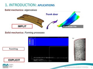
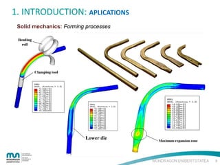
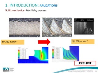
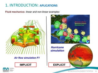
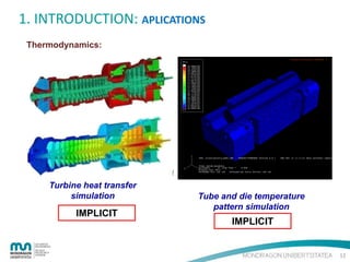
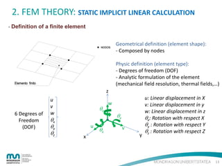
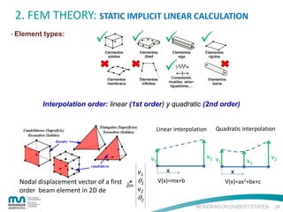
The document provides an introduction to the finite element method (FEM) for numerical analysis of engineering problems. It discusses how FEM can be used to solve complex problems by dividing them into smaller, simpler elements. FEM allows the use of computers to solve problems that cannot be solved through analytical methods. It also describes the different types of FEM formulations including implicit, which tries to obtain structural equilibrium at each time step for faster solutions, and explicit, which does not require iterations but has longer calculation times. Finally, the document gives examples of how FEM can be applied to problems in solid mechanics, fluid mechanics, and thermodynamics.

1. INTRODUCTION TO FINITE ELEMENT METHOD
(FEM)

2. 1. INTRODUCTION
ENGINEERING DEPARTMENT:
To develop new
products and/or manufacturing processes
Product calculation:
- Component dimensioning
- Design verification
- Material selection
Preliminary
design: concept
design
INDUSTRIALISATION:
- Development of manufacturing
Process calculation:
- Process parameters
drawings
- Manufacturing process
definition
- Development of manufacturing
tools
- Production
- Tooling design
2

3. 1. INTRODUCTION: CALCULATION METHODS
- Analytic method:
- Consists on the use of analytic equation to represent the behaviour of a
physical problem (As exercises solved by hand in previous chapters or other
subjects, heat transfer, material resistance, dynamics, vibrations,…)
- Advantages: relatively fast to be solved
- Limitations: Hard to represent complex phenomena in real components, not
always applicable.
3

4. 1. INTRODUCTION: CALCULATION METHODS
- Numeric methods (Finite Element Methods FEM)
- To divide a complex problem into many
simple problems (elements)
- Problem solution by numeric methods
(Newton-Raphson) by using iterations and
increments.
- Advantages: Capability to solve complex
problems.
- Limitations: Time expensive resolution
method, the use of computers is required.
4

5. 1. INTRODUCTION: FORMULATION TYPES
- Implicit:
- Tries to obtain the structural equilibrium for each time increment.
- More sophisticate algorithms
higher time increments (FASTER).
- High precision
- Convergence problems when solving non-linear phenomena: hard
variations in boundary condition, material behaviour, loads, contacts,…
- Explicit:
- Does not need iterations, just time increments (Does not try to get the
exact solution)
- No convergence problems
- Utilizes constant time increments
- High calculation time
- Recommendable to solve non-linear problems.
5

6. 1. INTRODUCTION: APLICATIONS
Solid mechanics:
- Structural linear calculations (linear static, linear dynamics) IMPLICIT
- Plasticity range calculation (no-linear quasi-static or dynamics) EXPLICIT
Fluid mechanics:
- Linear calculation (wind tunnel example) IMPLICIT
- Non-linear calculations (atmospheric phenomena, turbulence, wind,...) EXPLICIT
Thermodynamics: (linear problems-IMPLICIT)
Multiphysics: thermo mechanic, thermo fluidic, fluid structure
interaction…
6

7. 1. INTRODUCTION: APLICATIONS
Solid mechanics: Structural static calculation
Design
vs.
FEM
Set-up
IMPLICIT
Aluminium sheet bulge-test
7

8. 1. INTRODUCTION: APLICATIONS
Solid mechanics: eigenvalues
Trunk door
IMPLIT
First mode17Hz
Solid mechanics: Forming processes
Punching
EXPLICIT
8

9. 1. INTRODUCTION: APLICATIONS
Solid mechanics: Forming processes
9

10. 1. INTRODUCTION: APLICATIONS
Solid mechanics: Machining process
Vc=300 m.min-1
Vc≥600 m.min-1
EXPLICIT
10

11. 1. INTRODUCTION: APLICATIONS
Fluid mechanics: linear and non-linear examples
Hurricane
simulation
Air flow simulation F1
IMPLICIT
EXPLICIT
11

12. 1. INTRODUCTION: APLICATIONS
Thermodynamics:
Turbine heat transfer
simulation
IMPLICIT
Tube and die temperature
pattern simulation
IMPLICIT
12

13. 2. FEM THEORY: STATIC IMPLICIT LINEAR CALCULATION
- Definition of a finite element
Geometrical definition (element shape):
- Composed by nodes
Physic definition (element type):
- Degrees of freedom (DOF)
- Analytic formulation of the element
(mechanical field resolution, thermal fields,…)
z
6 Degrees of
Freedom
(DOF)
u
v
w
θx
θy
θz
θz
u
x
θx
w
θy
v
y
u: Linear displacement in X
v: Linear displacement in y
w: Linear displacement in z
θx: Rotation with respect X
θy : Rotation with respect Y
θz : Rotation with respect Z
13

14. 2. FEM THEORY: STATIC IMPLICIT LINEAR CALCULATION
- Element types:





Interpolation order: linear (1st order) y quadratic (2nd order)
Linear interpolation
v2 v
1
v1
v1
Nodal displacement vector of a first * θ1
δ= v
order beam element in 2D de
2
Quadratic interpolation
x
V(x)=mx+b
v3
v2
x
V(x)=ax2+bx+c
θ2
14

15. 2. FEM THEORY: STATIC IMPLICIT LINEAR CALCULATION
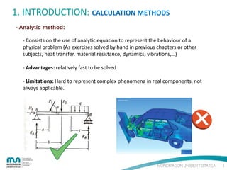
- Mechanical field calculation: Motion differential equation
.
..
[M]{δ} + [C]{δ}+[k]{δ} ={Fext}
[M]: Mass matrix
[C]: Damping matrix
[k]: Stiffness matrix
- Mechanical field: STATIC
Acceleration = 0
Velocity = 0
.
..
[M]{δ} + [C]{δ}+[k]{δ} ={Fext}
{δ}: Displacement vector
.
{δ}: Velocity vector
..
{δ}: Acceleration vector
{Fext}: External load vector
[k]{δ} ={Fext}
5 unknowns and 5 equations
15

16. 2. FEM THEORY: STATIC IMPLICIT LINEAR CALCULATION
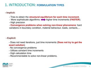
- Stress field calculation through nodal displacement.
Strain through local displacement
INTERPOLATION  displacement at
any point of the structure
 δ1 
 
 .
{ δ }e = [ N 1 , N 2 ,...., N n ]  
 .
 
δn 
Generalised Hooke’s law  Stress
calculation through local strain
(1 − ν)
 ν
σx 

σ 
 ν
 y

σz 
E
 
 0
 =
τ xy  (1 − 2 ⋅ ν) ⋅ (1 + ν) 
 0
τ yz 

 

τ zx 
 
 0

ν
(1 − ν)
ν
ν
0
0
0
0
(1 − 2ν)
2
0
0
ν
(1 − ν)
0
0
0
0
0
0
0
0
0
(1 − 2ν)
2
0

ε
0  x 
 ε 
0  y 
 ε 
0  z 
 
 γxy 
0  γyz 
 
(1 − 2ν) γzx 
 

2 
0





 εx  
 

 εy  
 

 εz  
 

=

γ xy  


 

 γ yz  
 

 γ zx  








∂
∂x
0
0
∂
∂y
0
0
∂
∂y
∂
∂x
0
∂
∂z
∂
∂z
0
0 



0 



∂ 
u
∂z  

 . v
0  
w
 


∂ 
∂y 


∂ 
∂x 






{ ε }= [ ∂ ] { δ }
ε3
ε1
ε2
16

17. 2. FEM THEORY: STATIC IMPLICIT LINEAR CALCULATION
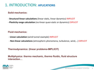
- INTERPOLATION FUNCTIONS: Determination of the displacement at any
point of the structure.
{δ }e = displacement vector at any point in a
{δ}e = [N]{δ* }e
determined element
{δ } = nodal displacement vector of a determined
*
e
{δ }e
 δ1 
= [N1 , N 2 ,..., N n ]  
δ n 
element
[N ] = interpolation function matrix
[Ni ] = interpolation function of the nodal
displacement a determined node i.
{δ i }
= displacement vector at a determined
node i.
So, the displacement at any point of a determined element is obtained:
{δ } = [N1 ]{δ1}+ [N 2 ]{δ 2 }+ ... + [N n ]{δ n }
Where [Nk] represents the contribution of node k’s displacement in the total displacement of
any determined point.
17

18. 2. FEM THEORY: STATIC IMPLICIT LINEAR CALCULATION
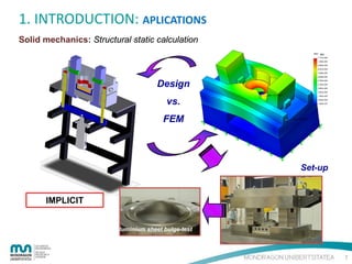
- STIFFNESS MATRIX:
{ }
{ }
In order to cause the nodal displacements δ * and consequently deform the element
it is necessary the presence of nodal forces f *
Definition: The stiffness coefficient Kij represents the necessary force to apply to a
certain degree of freedom i to obtain an unitary displacement of the degree of
freedom j being 0 the influence in the displacement of the rest of the degrees of
freedom
n
f i = ∑ K ij ⋅ δ j
j =1
n= number of DOF
K11 ⋅ δ1 + K12 ⋅ δ 2 + ... + K1n ⋅ δ n = f1

K n1 ⋅ δ1 + K n 2 ⋅ δ 2 + ... + K nn ⋅ δ n = f n
{ } = [K ] {δ }
Writing in matrix form: f
*
*
e
e
e
[K]e = Stiffness matrix of the element
18

19. 2. FEM THEORY: STATIC IMPLICIT LINEAR CALCULATION
DETERMINATION OF THE STIFFNESS MATRIX OF A FINITE ELEMENT
Relation between nodal forces an nodal displacements:
{f }= [K ]{δ }
*
*
Based on CAPLEYRON theory, the external work of the nodal forces is represented:
w=
1 *T *
{δ } {f }
2
w=
1 *T
{δ } [K ]{δ * }
2
1
T
σ
The internal deformation energy caused by the nodal displacements: u = ∫ {ε } { }⋅ dv
2
As: {ε } = ∂{δ } = ∂[N ]{ * }= [B]{ * }
1
δ
δ
}T   δ *
u = ∫ { [T [D ][ }⋅ dv
δ * B]  B]{ 
2v T
{σ } = [D]{ε } = [D][B]{δ * }
T
{ε }
Being  w = u
{ } [K ]{δ }
1 *
δ
2
T
*
{ }
1
= δ*
2
[K ] = ∫ [B ]T [D][B ]⋅ dv
T
{σ }

 *
T
 ∫ [B ] [D ][B ]⋅ dv  δ


v

{ }
STIFFNESS MATRIX
v
19

20. 2. FEM THEORY: STATIC IMPLICIT LINEAR CALCULATION
- DETERMINATION OF THE STIFFNESS MATRIX IN GLOBAL COORDINATES
Transformation matrix
a x
[T ] = bx

 cx

az 

bz 
cz 

ay
by
cy
From local coordinate
system of the element
To global coordinate system
{δ }= [T ]{δ }
*
{f }= [T ]{f }
{f }= [T ] {f }
*
*
{f }= [K ]{δ }
*
*
T
*
*
{f }= [K ]{δ }
*
*
*
{f }= [T ] {f }= [T ] [K ]{δ }= [T ] [K ][T ]{δ }
*
T
*
T
[K ] = [T ]T [K ][T ]
*
T
*
[K] in GLOBAL coord. system
20

21. 2. FEM THEORY: STATIC IMPLICIT LINEAR CALCULATION
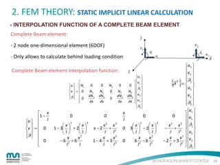
- INTERPOLATION FUNCTION OF A TRUSS ELEMENT
Truss element:
y
- 2 node one-dimensional element (2DOF)
u1
- Only allows to calculate tractive-compressive condition
Nodal displacement vector
{δ }= {u ,u }
T
1
1
i
u (x )
L
u2
2
j
x
x , y , z Local axis
i, j
Element nodes
2
Determination of the interpolation function
u1 , u2 Nodal displacements
2 G.D.L  1st order equation u ( x ) = a0 + a1.x
u (0) = u1
u (l ) = u2
}u = a + a l}
u1 = a0
2
a0 = u1
1
1
a1 = − u1 + u2
l
l
}
0
u1 
u = [N1 , N 2 ] 
u2 
u1  1 0  a0 
 =
 
u 2  1 l  a1 


1
a0  1 l
 = 
a1  l − 1
0 u1 
 
1 u2 

N1 = 1 −
x
l
0
1
 − 1 1  u1  = 1 − x , x  u1 
u = [1, x ]


 
 u2  

l  l  u2 

  
 l l
N2 =
x
l
21

22. 2. FEM THEORY: STATIC IMPLICIT LINEAR CALCULATION
- STIFFNESS MATRIX OF A TRUSS ELEMENT
Truss element: 2DOF
y
u1
u2
1
2
L
{δ }
*
x ,y
x
u1 
= 
u2  x ,y
u   x
ux ,y = [N1 N2 ] 1  = 1 −
u2   l
u1   ∂N1 ∂N2  u1   1 1  u1 
∂u  ∂ 
,
ε x = =  [N1 , N2 ]  = 
 = − ,  
u2   ∂x ∂x  u2   l l  u2 
∂x  ∂x 

 



[B ]
x
N2 =
l
x
l
Local coordinate system
[B ]
Stiffness matrix obtaining formula:
[k ] = ∫ [B] [D][B].dv
[N ] = [N1 ,N2 ]
N1 = 1 −
x  u1 
 
l  u2 

T
v
1
 1
 1
− 
− 2
l
 l  1 1
 l2
l dx = E.S 1 − 1
K = ∫  E − , .dv = S.E ∫ 
.
1
1
1   l l
l − 1 1


v 
0 −
2
2 
 l 

l 
 
 l
[]
22

23. 2. FEM THEORY: STATIC IMPLICIT LINEAR CALCULATION
- STIFFNESS MATRIX OF A TRUSS ELEMENT
[k ] = EL.S −11

e

− 1
1

Stiffness matrix of TRUSS element
in local coordinate system
- RIGIDITY MATRIX OF A TRUSS ELEMENT IN GLOBAL COORD. SYSTEM

y
y
Displacement vector in global axis:

u1

x
ϑ
x
cosθ
u1 
 sinθ
v 
 1
u  = 
 0
 2
v2  X ,Y  0
 

− sinθ
cosθ
0
0
cosθ
0
sinθ
0
0
 u1 
0  0 
 
 
− sinθ  v1 

cosθ  0  x ,y
 
23

24. 2. FEM THEORY: STATIC IMPLICIT LINEAR CALCULATION
- STIFFNESS MATRIX OF A TRUSS ELEMENT IN GLOBAL COORD. SYSTEM
Naming
µ = senϑ 

λ = cosϑ 
[K ]e = [T ]T [K ] [T ]
λ − µ 0 0  1


E.S  µ λ 0 0  0
[K ]e =
l 0 0 λ − µ   − 1


0 0 µ λ  0

λ2
λµ

µ2
E.S  µλ
[K ]e =  2
l −λ
− λµ

− λµ − µ 2

− λ2
− λµ
λ2
µλ
− λµ 
2
−µ 
λµ 

2
µ 

0 − 1 0  λ
0 0 0  − µ

0 1 0  0

0 0 0  0
µ 0
λ 0
0 λ
0 −µ
0
0

µ

λ
Stiffness matrix of a TRUSS
element in GLOBAL coordinate
system
24

25. 2. FEM THEORY: STATIC IMPLICIT LINEAR CALCULATION
- INTERPOLATION FUNCTION OF A BEAM ELEMENT
Beam element:
y
- 2 node unidimensional element (4DOF)
v1
- Only allows to calculate behind loading condition
z
Beam element interpolation function:
N
v   1
  =  dN1
ϑ  
 dx
2
3

 x
 x
1 − 3  + 2  ,
v  
l
l
 =
ϑ  
x
x2
 −6 2 +6 ,
l
l

N2
N3
dN 2 dN 3
dx
dx
v1 
N4  
ϑ1 
dN 4   
 v2

dx   
ϑ2 
 
x 2 x3
x−2 + 2 ,
l l
x
x2
1− 4 + 3 2 ,
l
l
v2
ϑ1
ϑ2

x
v1 
ϑ 
 
=  1
v2 
ϑ2 
 
{δ }
T
2
3
x 2 x 3  v1 
 x
 x
3  − 2  , − + 2   
l l  ϑ1 
l
l
 
x
x2
x
x 2  v2 
6 2 −6 3 ,
− 2 + 3 2  
l
l
l
l  ϑ2 
25

26. 2. FEM THEORY: STATIC IMPLICIT LINEAR CALCULATION
- INTERPOLATION FUNCTION OF A COMPLETE BEAM ELEMENT
Complete Beam element:
y
- 2 node one-dimensional element (6DOF)
v1
- Only allows to calculate behind loading condition
Complete Beam element interpolation function:

u  N1
  
v  =  0
ϑ  
 
0


 x
1 − l
u  
  
v  = 0
ϑ  
  
 0

0
N3
dN3
dx
0
2
x
x
1 − 3  + 2 
l
l
x
x2
−6 2 +6
l
l
0
N4
dN4
dx
N2
0
0
0
3
x2 x3
x −2 + 2
l
l
x
x2
1−4 +3 3
l
l
v2
ϑ1
ϑ2 u
2
u1
x
z
u1 
 v1 
0  
 
ϑ1 
N6   

dN6  u2 
dx  v2 
 
ϑ2 
 
0
N5
dN5
dx
x
l
0
0
{δ }
T
0
2
x
x
3  − 2 
l
l
x
x2
6 2 −6 3
l
l
u1 
v 
 1
ϑ 
 
=  1
u2 
v2 
 
 
ϑ2 
3
u 
 1 
0
 v1 

x 2 x 3  ϑ1 
 
− + 2  
l
l  u2 
x
x 2  v 
− 2 + 3 2  2 
l
l  ϑ 
 2
26

27. 2. FEM THEORY: STATIC IMPLICIT LINEAR CALCULATION
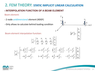
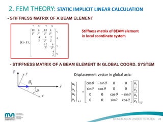
- STIFFNESS MATRIX OF A BEAM ELEMENT
BEAM element: 4 DOF
dv
dθ
d 2v
εx = −y
= − y 2 being θ =
dx
dx
dx
Beam deflection
( { })
{ }
d 2v
d2
ε x = − y 2 = − y 2 [N ] δ * = [B ] δ *
dx
dx
{δ }
*
x, y
 v1 
θ 
 
=  1
v
 2
θ 2  x , y
 
[N ] = [N1 , N2 , N3 , N4 ]
Local coordinate system
[B] = − y − 62 + 12 x3 , − 4 + 6 x2 ,

 l
l
l
l
6
x
2
x
− 12 3 , − + 6 2 
l2
l
l
l 
[k ] = ∫ [B]T [D][B]dv =
v
x
 6
− l 2 + 12 l 3 


− 4 + 6 x 
l
 l
x 4
x 6
x 2
x
l 2  6
2
= E∫ 
 − 2 + 12 3 , − + 6 2 , 2 − 12 3 ,− + 6 2  dx ∫ y ds
6
x
l
l
l
l l
l
l
l  s
0 
− 12 3  
l 2
l 
 2
x 
− + 6 2 
l 
 l
27

28. 2. FEM THEORY: STATIC IMPLICIT LINEAR CALCULATION
- STIFFNESS MATRIX OF A BEAM ELEMENT
Stiffness matrix of BEAM element
in local coordinate system
- STIFFNESS MATRIX OF A BEAM ELEMENT IN GLOBAL COORD. SYSTEM

y
y
Displacement vector in global axis:

u1

x
ϑ
x
cosθ
u1 
 sinθ
v 
 1
u  = 
 0
 2
v2  X ,Y  0
 

− sinθ
cosθ
0
0
0
0
cosθ
sinθ
0  u1 
 
0  v 1 
 
− sinθ  u2 

cosθ  v2 
  x ,y
28

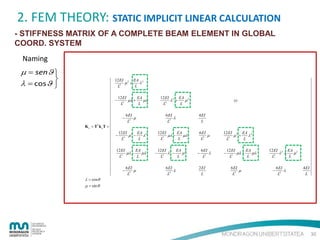
29. 2. FEM THEORY: STATIC IMPLICIT LINEAR CALCULATION
- STIFFNESS MATRIX OF A BEAM ELEMENT IN GLOBAL COORD. SYSTEM
Naming
µ = senϑ 

λ = cosϑ 
λ
− µ

0
[k ]e = E.Iz 
0
0


0
12 2
 l3 µ

 − 12 λ
 l3

− 6 µ
2
[k ]e = E.I z  l
 − 12
 3 µ2
 l
12
 3 λµ
l
− 6
 l3 µ

12 2
λ
l3
6
λ
l2
12
λµ
l3
− 12 2
λ
l3
6
l2
µ 0 0 0
λ 0 0 0
0
0
0
0
1 0
0λ
0− µ
0 0
0
µ
λ
0
0

0  0

0 
 0
0 

0  0

0 
 0
1 


0

4
l
6
12 2
µ
µ
2
l
l3
−6
− 12
λ
λµ
2
l
l3
2
−6
µ
l
l
0
12
l3
6
l2
0
− 12
l3
6
l2
12 2
λ
l3
−6
µ
l2
0 0 0
− 12
6
0 3
2
l
l
−6
4
0
l2
l
0 0 0
−6
12
0 3
l2
l
−6
2
0 2
l
l














4

l
0 
6 

l2  
2 

l 

0 

−6 

l2  

4 

l 
λ −µ 0 0 0 0
µ λ 0 0 0 0

0
0
0
0
0
0
0
0
1
0
0
0
0 0 0

λ − µ 0
µ λ 0

0 0 1

Stiffness matrix of a BEAM
element in GLOBAL coordinate
system
29

30. 2. FEM THEORY: STATIC IMPLICIT LINEAR CALCULATION
- STIFFNESS MATRIX OF A COMPLETE BEAM ELEMENT IN GLOBAL
COORD. SYSTEM
Naming
µ = senϑ 

λ = cosϑ 
12 EI 2 EA 2
µ +
λ
L3
L
−
12 EI
EA
µλ +
µλ
3
L
L
−
12 EI 2 EA 2
λ +
µ
L3
L
6 EI
µ
L2
6 EI
λ
L2
sy.
4 EI
L
= TT k e T
Ke =
−
12 EI 2 EA 2
µ −
λ
L3
L
12 EI
EA
µλ −
µλ
L3
L
−
6 EI
µ
L2
12 EI
EA
µλ −
µλ
L3
L
−
12 EI 2 EA 2
λ −
µ
L3
L
6 EI
λ
L2
6 EI
µ
L2
−
6 EI
λ
L2
2 EI
L
12 EI 2 EA 2
µ +
λ
L3
L
−
12 EI
EA
µλ +
µλ
L3
L
6 EI
µ
L2
12 EI 2 EA 2
λ +
µ
L3
L
−
6 EI
λ
L2
4 EI
L
λ = cos θ
µ = sin θ
30

31. 2. FEM THEORY: STATIC IMPLICIT LINEAR CALCULATION
- DETERMINATION THE EQUIVALENT NODAL LOAD VECTOR
In a real problem different type of external loads can be found:
- Punctual forces
- Moments
- Distributed loads
For FEM modelling all
external load should be
applied in the element
nodes


- Punctual forces
- Moments
- Distributed loads
NECESITY TO OBTAIN AN EQUIVALENT SYSTEM BASED
IN NODAL LOADS
f
=
f*
31

32. 2. FEM THEORY: STATIC IMPLICIT LINEAR CALCULATION
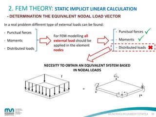
- DETERMINATION THE EQUIVALENT NODAL LOAD VECTOR
The external work due to all the external load applied to the system is given by
1
T
w1 = ∫ {δ } { f }⋅ ds
2s
By using the interpolation functions:
w1 =
{ } [N ] { f }⋅ ds = 1 {δ } ∫ [N ] { f }⋅ ds
2
1
δ*
2∫
s
T
* T
T
T
s
Thus the work of the equivalent system can be written as:
w2 =
w1 = w2
{ } {f }
1 *
δ
2
T
*
{ } ∫ [N ] { f }⋅ ds = 1 {δ } {f }
2
1 *
δ
2
T
* T
T
*
s
{f }= ∫ [N ] { f }⋅ ds
T
*
s
32

33. 2. FEM THEORY: STATIC IMPLICIT LINEAR CALCULATION
DETERMINATION OF THE STRESS/STRAIN CONDITION:
Once, the nodal displacement vector of the studied system is solved the stress/strain
condition at any point can be obtained.
STEP 1: STRAIN DETERMINATION AT A CERTAIN POINT
 δ1 
 
 .
{ δ }e = [ N 1 , N 2 ,...., N n ]  
 .
 
δn 
Determination of
the elongation at
the selected point
{ε } = [∂ ]{δ }
{ε } = ∂[N ]{δ * }= [B]{δ * }


εx  
ε  
 y 
εz  
 
 =
γ xy  
γ yz  
  
γ zx  
 


∂
∂x
0
0
∂
∂y
0
∂
∂z
0
∂
∂y
0
∂
∂
∂x
∂z
0
0 

0 

∂ u 
∂ z  
 v 
0  
  w
∂ 
∂y

∂ 
∂x 
Strain vector determination
33

34. 2. FEM THEORY: STATIC IMPLICIT LINEAR CALCULATION
DETERMINATION OF THE STRESS/STRAIN CONDITION:
STEP 2: STRESS DETERMINATION AT A CERTAIN POINT
The relation between the strain and the stress in the linear elastic domain is given by
the generalised Hooke’s law:
[
]
[
]
[
]
1
σ x − υ (σ y + σ z )
E
1
ε y = σ y − υ (σ z + σ x )
E
1
ε z = σ z − υ (σ x + σ y )
E
εx =
2(1 + υ )
τ xy
G
E
τ
2(1 + υ )
τ yz
γ yz = yz =
G
E
τ
2(1 + υ )
γ zx = zx =
τ zx
G
E
γ xy =
τ xy
=
Generalized Hooke’s law
LAMÉ ' s _ law : G =
E
 For isotropic materials
2(1 + υ )
34

35. 2. FEM THEORY: STATIC IMPLICIT LINEAR CALCULATION
DETERMINATION OF THE STRESS/STRAIN CONDITION:
STEP 2: STRESS DETERMINATION AT A CERTAIN POINT
The relation between the strain and the stress in the linear elastic domain is given by
the generalized Hooke’s law:
0
0
0 
υ
(1 − υ ) υ
 υ (1 − υ ) υ
0
0
0  ε
 x 

σ x 
 υ
σ 
0
0  ε 
υ (1 − υ ) 0
y
 y 


 1 − 2υ 
 0
σ z 
0
0 
0  ε z 
E
 0
 
 

 
 =
 2 
τ xy  (1 − 2υ )(1 + υ ) 
 γ xy 

 1 − 2υ 

 0
τ yz 
0
0
0
 0  γ yz 


 
 
 2 
 γ 

τ zx 
 
 1 − 2υ   zx 

0
0
0
0 

 0
2 



{σ } = [D]{ε }
35