This document outlines the contents and concepts of a course on finite element analysis. It covers fundamental concepts like discretization, matrix algebra, and weighted residual methods. It also covers one-dimensional problems involving bars, beams, and trusses. Shape functions, stiffness matrices, and finite element equations are derived for one-dimensional elements. Two-dimensional problems involving plane stress, strain, and heat transfer are also introduced. Numerical integration techniques are discussed. A variety of finite element applications are listed including structural and non-structural problems.

1. ME1401 – INTRODUCTION OF FINITE ELEMENT ANALYSIS
CONTENTS
UNIT – I
Fundamental Concepts
Syllabus
General Methods of the Finite Element Analysis
General Steps of the Finite Element Analysis
Boundary Conditions
Consideration during Discretization process
Rayleigh – Ritz Method (Variational Approach)
Problems (I set)
Weighted Residual method
Problems (II set)
Matrix Algebra
Matrix Operation
Gaussian Elimination Method
Problems (III set)
Advantages of Finite Element Method
Disadvantages of Finite Element Method
Applications of Finite Element Analysis
UNIT – II
One Dimension Problems
Syllabus
One Dimensional elements
Bar, Beam and Truss
Stress, Strain and Displacement
Types of Loading
Finite Element Modeling
Co – Ordinates

2. Natural Co – Ordinate (ε)
Shape function
Polynomial Shape function
Stiffness Matrix [K]
Properties of Stiffness Matrix
Equation of Stiffness Matrix for One dimensional bar element
Finite Element Equation for One dimensional bar element
The Load (or) Force Vector {F}
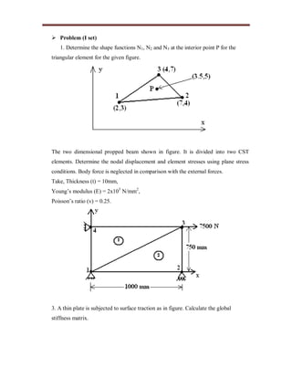
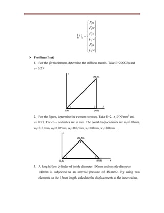
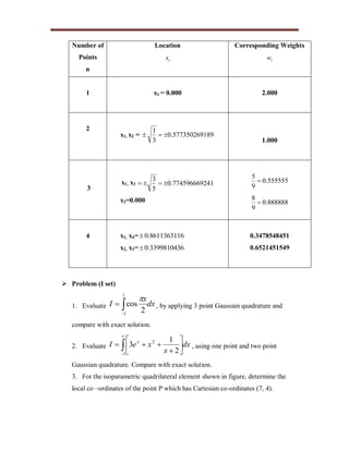
Problem (I set)
Trusses
Stiffness Matrix [K] for a truss element
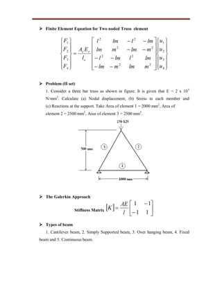
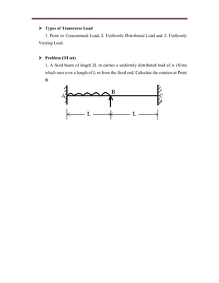
Finite Element Equation for Two noded Truss element
Problem (II set)
The Galerkin Approach
Types of beam
Types of Transverse Load
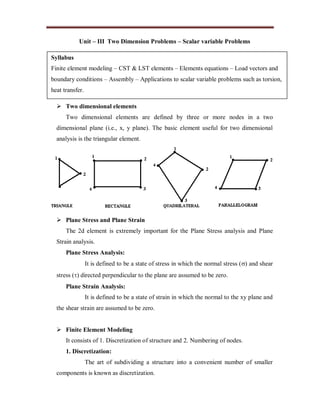
Problem (III set)
UNIT – III
Two Dimension Problems – Scalar variable Problems
Syllabus
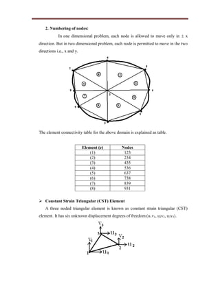
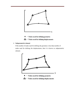
Two dimensional elements
Plane Stress and Plane Strain
Finite Element Modeling
Constant Strain Triangular (CST) Element
Shape function for the CST element
Displacement function for the CST element
Strain – Displacement matrix [B] for CST element
Stress – Strain relationship matrix (or) Constitutive matrix [D] for two dimensional
element
Stress – Strain relationship matrix for two dimensional plane stress problems

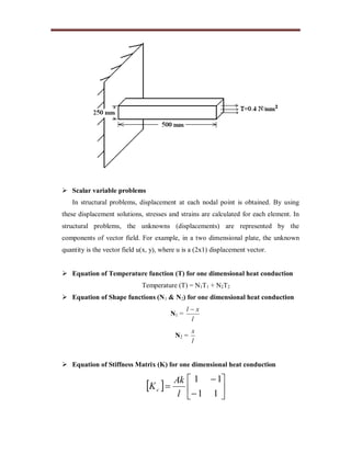
3. Stress – Strain relationship matrix for two dimensional plane strain problems
Stiffness matrix equation for two dimensional element (CST element)
Temperature Effects
Galerkin Approach
Linear Strain Triangular (LST) element
Problem (I set)
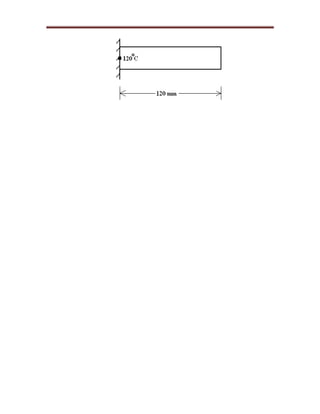
Scalar variable problems
Equation of Temperature function (T) for one dimensional heat conduction
Equation of Shape functions (N1 & N2) for one dimensional heat conduction
Equation of Stiffness Matrix (K) for one dimensional heat conduction
Finite Element Equations for one dimensional heat conduction
Finite element Equation for Torsional Bar element
Problem (II set)
UNIT – IV
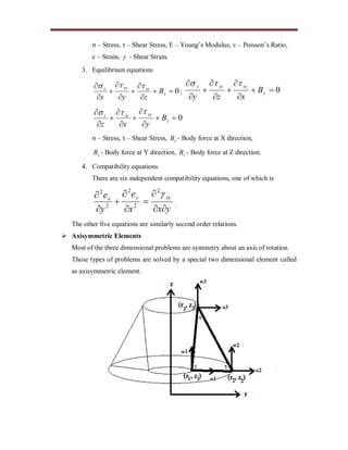
AXISYMMETRIC CONTINUUM
Syllabus
Elasticity Equations
Axisymmetric Elements
Axisymmetric Formulation
Equation of shape function for Axisymmetric element
Equation of Strain – Displacement Matrix [B] for Axisymmetric element
Equation of Stress – Strain Matrix [D] for Axisymmetric element
Equation of Stiffness Matrix [K] for Axisymmetric element
Temperature Effects
Problem (I set)

4. UNIT – V
ISOPARAMETRIC ELEMENTS FOR TWO DIMENSIONAL CONTINUUM
Syllabus
Isoparametric element
Superparametric element
Subparametric element
Equation of Shape function for 4 noded rectangular parent element
Equation of Stiffness Matrix for 4 noded isoparametric quadrilateral element
Equation of element force vector
Numerical Integration (Gaussian Quadrature)
Problem (I set)

5. ME 1401 INTRODUCTION OF FINITE ELEMENT ANALYSIS
Unit – I Fundamental Concepts
Syllabus
Historical background – Matrix approach – Application to the continuum –
Discretisation – Matrix algebra – Gaussian elimination – Governing equations for
continuum – Classical Techniques in FEM – Weighted residual method – Ritz
method
 General Methods of the Finite Element Analysis
1. Force Method – Internal forces are considered as the unknowns of the problem.
2. Displacement or stiffness method – Displacements of the nodes are considered
as the unknowns of the problem.
 General Steps of the Finite Element Analysis
Discretization of structure > Numbering of Nodes and Elements > Selection of
Displacement function or interpolation function > Define the material behavior by
using Strain – Displacement and Stress – Strain relationships > Derivation of
element stiffness matrix and equations > Assemble the element equations to
obtain the global or total equations > Applying boundary conditions > Solution
for the unknown displacements > computation of the element strains and stresses
from the nodal displacements > Interpret the results (post processing).
 Boundary Conditions
It can be either on displacements or on stresses. The boundary conditions on
displacements to prevail at certain points on the boundary of the body, whereas
the boundary conditions on stresses require that the stresses induced must be in
equilibrium with the external forces applied at certain points on the boundary of
the body.
 Consideration During Discretization process
Types of element > Size of element > Location of node > Number of elements.

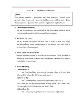
6.  Rayleigh – Ritz Method (Variational Approach)
It is useful for solving complex structural problems. This method is possible only
if a suitable functional is available. Otherwise, Galerkin’s method of weighted
residual is used.
 Problems (I set)
1. A simply supported beam subjected to uniformly distributed load over entire
span. Determine the bending moment and deflection at midspan by using
Rayleigh – Ritz method and compare with exact solutions.
2. A bar of uniform cross section is clamed at one end and left free at another end
and it is subjected to a uniform axial load P. Calculate the displacement and stress
in a bar by using two terms polynomial and three terms polynomial. Compare
with exact solutions.
 Weighted Residual method
It is a powerful approximate procedure applicable to several problems. For non –
structural problems, the method of weighted residuals becomes very useful. It has
many types. The popular four methods are,
1. Point collocation method,
Residuals are set to zero at n different locations Xi, and the weighting function wi
is denoted as (x - xi).
)( xix   R (x; a1, a2, a3… an) dx = 0
2. Subdomain collocation method,
w1 =



10
11
forxnotinD
forxinD
3. Least square method,
 [R (x; a1, a2, a3… an)]2
dx = minimum.
4. Galerkin’s method.
wi = Ni (x)
 Ni (x) [R (x; a1, a2, a3… an)]2
dx = 0, i = 1, 2, 3, …n.

7.  Problems (II set)
1. The following differential equation is available for a physical phenomenon.
2
2
dx
yd + 50 = 0, 0  x 10. Trial function is y = a1x (10-x). Boundary conditions
are y (0) = 0 and y (10) = 0. Find the value of the parameter a1 by the following
methods, (1) Point collocation method, (2) Subdomain collocation method, (3)
Least square method and (4) Galerkin’s method.
2. The differential equation of a physical phenomenon is given by
2
2
dx
yd
- 10x2
= 5. Obtain two term Galerkin solution b using the trial functions:
N1(x) = x(x-1); N2(x) = x2
(x-1); 0  x 1. Boundary conditions are y (0) = 0 and
y (1) = 0.
 Matrix Algebra
Equal matrix: Two matrixes are having same order and corresponding elements
are equal.
Diagonal matrix: Square matrix in which all the elements other than the diagonal
are zero.
Scalar matrix: Square matrix in which all the elements are equal.
Unit matrix: All diagonal elements are unity and other elements are zero.
 Matrix Operation
Scalar multiplication, Addition and Subtraction of matrices, Multiplication of
matrices, Transpose of a matrix, Determinant of a matrix, inverse of a matrix,
Cofactor or Adjoint method to determine the inverse of a matrix, Row reduction
method (Gauss Jordan method) to determine the inverse of a matrix, Matrix
differentiation and matrix integration.
 Gaussian Elimination Method
It is most commonly used for solving simultaneous linear equations. It is easily
adapted to the computer for solving such equations.

8.  Problems (III set)
1. 3x+y-z = 3, 2x-8y+z = -5, x-2y+9z = 8. Solve by using Gauss – Elimination
method.
2. 2a+4b+2c = 15, 2a+b+2c = -5, 4a+b-2c = 0. Solve the equations by using
Gauss – Elimination method.
 Advantages of Finite Element Method
1. FEM can handle irregular geometry in a convenient manner.
2. Handles general load conditions without difficulty
3. Non – homogeneous materials can be handled easily.
4. Higher order elements may be implemented.
 Disadvantages of Finite Element Method
1. It requires a digital computer and fairly extensive
2. It requires longer execution time compared with FEM.
3. Output result will vary considerably.
 Applications of Finite Element Analysis
Structural Problems:
1. Stress analysis including truss and frame analysis
2. Stress concentration problems typically associated with holes, fillets or
other changes in geometry in a body.
3. Buckling Analysis: Example: Connecting rod subjected to axial
compression.
4. Vibration Analysis: Example: A beam subjected to different types of
loading.
Non - Structural Problems:
1. Heat Transfer analysis:
Example: Steady state thermal analysis on composite cylinder.
2. Fluid flow analysis:
Example: Fluid flow through pipes.

9. Unit – II One Dimension Problems
Syllabus
Finite element modeling – Coordinates and shape functions- Potential energy
approach – Galarkin approach – Assembly of stiffness matrix and load vector – Finite
element equations – Quadratic shape functions – Applications to plane trusses
 One Dimensional elements
Bar and beam elements are considered as One Dimensional elements. These
elements are often used to model trusses and frame structures.
 Bar, Beam and Truss
Bar is a member which resists only axial loads. A beam can resist axial, lateral
and twisting loads. A truss is an assemblage of bars with pin joints and a frame is
an assemblage of beam elements.
 Stress, Strain and Displacement
Stress is denoted in the form of vector by the variable x as σx, Strain is denoted in
the form of vector by the variable x as ex, Displacement is denoted in the form of
vector by the variable x as ux.
 Types of Loading
(1) Body force (f)
It is a distributed force acting on every elemental volume of the body. Unit
is Force / Unit volume. Ex: Self weight due to gravity.
(2) Traction (T)
It is a distributed force acting on the surface of the body. Unit is
Force / Unit area. But for one dimensional problem, unit is Force / Unit length.
Ex: Frictional resistance, viscous drag and Surface shear.
(3) Point load (P)
It is a force acting at a particular point which causes displacement.

10.  Finite Element Modeling
It has two processes.
(1) Discretization of structure
(2) Numbering of nodes.
 CO – ORDINATES
(A) Global co – ordinates, (B) Local co – ordinates and (C) Natural co –
ordinates.
 Natural Co – Ordinate (ε)
ε =





 
2
12 xx
pc
Integration of polynomial terms in natural co – ordinates for two dimensional
elements can be performed by using the formula,
     
 
AXdALLL 2
!
!!!
321




 Shape function
N1N2N3 are usually denoted as shape function. In one dimensional problem, the
displacement
u =  Ni ui =N1 u1
For two noded bar element, the displacement at any point within the element is
given by,
u =  Ni ui =N1 u1 + N2 u2
For three noded triangular element, the displacement at any point within the
element is given by,

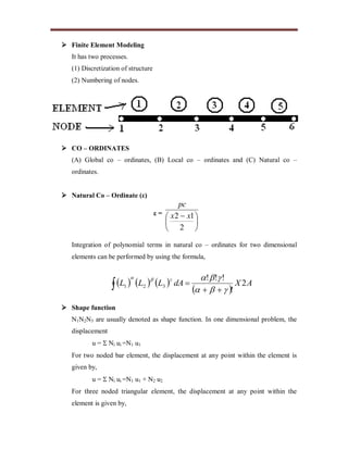
11. u =  Ni ui =N1 u1 + N2 u2 + N3 u3
v =  Ni vi =N1 v1 + N2 v2 + N3 v3
Shape function need to satisfy the following
(a) First derivatives should be finite within an element; (b) Displacement should
be continuous across the element boundary.
 Polynomial Shape function
Polynomials are used as shape function due to the following reasons,
(1) Differentiation and integration of polynomials are quite easy.
(2) It is easy to formulate and computerize the finite element equations.
(3) The accuracy of the results can be improved by increasing the order of the
polynomial.
 Stiffness Matrix [K]
Stiffness Matrix [K] =     dvBDB
T
V

 Properties of Stiffness Matrix
1. It is a symmetric matrix, 2. The sum of elements in any column must be equal
to zero, 3. It is an unstable element. So the determinant is equal to zero.
 Equation of Stiffness Matrix for One dimensional bar element
[K] = 







11
11
l
AE
 Finite Element Equation for One dimensional bar element





















2
1
2
1
11
11
u
u
l
AE
F
F

12.  The Load (or) Force Vector {F}
 







1
1
2
Al
F e

 Problem (I set)
1. A two noded truss element is shown in figure. The nodal displacements are
u1 = 5 mm and u2 = 8 mm. Calculate the displacement at x = ¼, 1/3 and ½.
 Trusses
It is made up of several bars, riveted or welded together. The following
assumptions are made while finding the forces in a truss,
(a) All members are pin joints, (b) The truss is loaded only at the joints, (c) The
self – weight of the members is neglected unless stated.
 Stiffness Matrix [K] for a truss element
 



















22
22
22
22
mlmmlm
lmllml
mlmmlm
lmllml
l
EA
K
e
ee

13.  Finite Element Equation for Two noded Truss element















































4
3
2
1
22
22
22
22
4
3
2
1
u
u
u
u
mlmmlm
lmllml
mlmmlm
lmllml
l
EA
F
F
F
F
e
ee
 Problem (II set)
1. Consider a three bar truss as shown in figure. It is given that E = 2 x 105
N/mm2
. Calculate (a) Nodal displacement, (b) Stress in each member and
(c) Reactions at the support. Take Area of element 1 = 2000 mm2
, Area of
element 2 = 2500 mm2
, Area of element 3 = 2500 mm2
.
 The Galerkin Approach
Stiffness Matrix   








11
11
l
AE
K
 Types of beam
1. Cantilever beam, 2. Simply Supported beam, 3. Over hanging beam, 4. Fixed
beam and 5. Continuous beam.

14.  Types of Transverse Load
1. Point or Concentrated Load, 2. Uniformly Distributed Load and 3. Uniformly
Varying Load.
 Problem (III set)
1. A fixed beam of length 2L m carries a uniformly distributed load of w (N/m)
which runs over a length of L m from the fixed end. Calculate the rotation at Point
B.

15. Unit – III Two Dimension Problems – Scalar variable Problems
 Two dimensional elements
Two dimensional elements are defined by three or more nodes in a two
dimensional plane (i.e., x, y plane). The basic element useful for two dimensional
analysis is the triangular element.
 Plane Stress and Plane Strain
The 2d element is extremely important for the Plane Stress analysis and Plane
Strain analysis.
Plane Stress Analysis:
It is defined to be a state of stress in which the normal stress () and shear
stress () directed perpendicular to the plane are assumed to be zero.
Plane Strain Analysis:
It is defined to be a state of strain in which the normal to the xy plane and
the shear strain are assumed to be zero.
 Finite Element Modeling
It consists of 1. Discretization of structure and 2. Numbering of nodes.
1. Discretization:
The art of subdividing a structure into a convenient number of smaller
components is known as discretization.
Syllabus
Finite element modeling – CST & LST elements – Elements equations – Load vectors and
boundary conditions – Assembly – Applications to scalar variable problems such as torsion,
heat transfer.

16. 2. Numbering of nodes:
In one dimensional problem, each node is allowed to move only in  x
direction. But in two dimensional problem, each node is permitted to move in the two
directions i.e., x and y.
The element connectivity table for the above domain is explained as table.
Element (e) Nodes
(1) 123
(2) 234
(3) 435
(4) 536
(5) 637
(6) 738
(7) 839
(8) 931
 Constant Strain Triangular (CST) Element
A three noded triangular element is known as constant strain triangular (CST)
element. It has six unknown displacement degrees of freedom (u1v1, u2v2, u3v3).

17.  Shape function for the CST element
Shape function N1 = (p1 + q1x + r1y) / 2A
Shape function N2 = (p2 + q2x + r2y) / 2A
Shape function N3 = (p3 + q3x + r3y) / 2A
 Displacement function for the CST element
Displacement function u =

































3
3
2
2
1
1
302010
030201
),(
),(
v
u
v
u
v
u
X
NNN
NNN
yxv
yxu
 Strain – Displacement matrix [B] for CST element
Strain – Displacement matrix [B] =










332211
321
321
000
000
2
1
qrqrqr
rrr
qqq
A
Where, q1 = y2 – y3 r1 = x3 – x2
q2 = y3 – y1 r2 = x1 – x3
q3 = y1 – y2 r3 = x2 – x1
 Stress – Strain relationship matrix (or) Constitutive matrix [D] for two
dimensional element
[D] =
   





































2
21
00000
0
2
21
0000
00
2
21
000
0001
0001
0001
211
v
v
v
vvv
vvv
vvv
vv
E

18.  Stress – Strain relationship matrix for two dimensional plane stress problems
The normal stress z and shear stresses xz, yz are zero.
[D] =













2
1
00
01
01
1 2
v
v
v
v
E
 Stress – Strain relationship matrix for two dimensional plane strain
problems
Normal strain ez and shear strains exz, eyz are zero.
[D] =
   
















2
21
00
0)1(
0)1(
211 v
vv
vv
vv
E
 Stiffness matrix equation for two dimensional element (CST element)
Stiffness matrix [k] = [B]T
[D] [B] A t
[B] =










332211
321
321
000
000
2
1
qrqrqr
rrr
qqq
A
For plane stress problems,
[D] =













2
1
00
01
01
1 2
v
v
v
v
E
For plane strain problems,

19. [D] =
   
















2
21
00
0)1(
0)1(
211 v
vv
vv
vv
E
 Temperature Effects
Distribution of the change in temperature (ΔT) is known as strain. Due to the
change in temperature can be considered as an initial strain e0.
σ = D (Bu - e0)
 Galerkin Approach
Stiffness matrix [K]e = [B]T
[D][B] A t.
Force Vector {F}e = [K]e {u}
 Linear Strain Triangular (LST) element
A six noded triangular element is known as Linear Strain Triangular (LST)
element. It has twelve unknown displacement degrees of freedom. The displacement
functions of the element are quadratic instead of linear as in the CST.

20.  Problem (I set)
1. Determine the shape functions N1, N2 and N3 at the interior point P for the
triangular element for the given figure.
The two dimensional propped beam shown in figure. It is divided into two CST
elements. Determine the nodal displacement and element stresses using plane stress
conditions. Body force is neglected in comparison with the external forces.
Take, Thickness (t) = 10mm,
Young’s modulus (E) = 2x105
N/mm2
,
Poisson’s ratio (v) = 0.25.
3. A thin plate is subjected to surface traction as in figure. Calculate the global
stiffness matrix.

21.  Scalar variable problems
In structural problems, displacement at each nodal point is obtained. By using
these displacement solutions, stresses and strains are calculated for each element. In
structural problems, the unknowns (displacements) are represented by the
components of vector field. For example, in a two dimensional plate, the unknown
quantity is the vector field u(x, y), where u is a (2x1) displacement vector.
 Equation of Temperature function (T) for one dimensional heat conduction
Temperature (T) = N1T1 + N2T2
 Equation of Shape functions (N1 & N2) for one dimensional heat conduction
N1 =
l
xl 
N2 =
l
x
 Equation of Stiffness Matrix (K) for one dimensional heat conduction
  








11
11
l
Ak
Kc

22.  Finite Element Equations for one dimensional heat conduction
Case (i): One dimensional heat conduction with free end convection


































1
0
10
00
11
11
2
1
AhT
T
T
hA
l
Ak
Case (ii): One dimensional element with conduction, convection and internal heat
generation.
































 
1
1
221
12
611
11
2
1 lPhTQAl
T
ThPl
l
Ak
 Finite element Equation for Torsional Bar element





















x
x
x
x
l
GJ
M
M
2
1
2
1
11
11


Where, Stiffness matrix [K] = 







11
11
l
GJ
 Problem (II set)
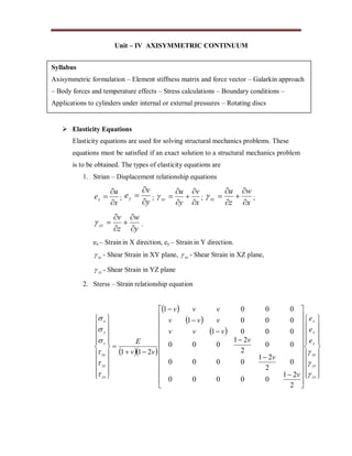
1. An Aluminium alloy fin of 7 mm thick and 50 mm long protrudes from a wall,
which is maintained at 120°C. The ambient air temperature is 22°C. The heat
transfer coefficient and thermal conductivity of fin material are 140 W/m2
K and 55
W/mK respectively. Determine the temperature distribution of fin.
2. Calculate the temperature distribution in a one dimension fin with physical
properties given in figure. The fin is rectangular in shape and is 120 mm long, 40mm
wide and 10mm thick. Assume that convection heat loss occurs from the end of the
fin. Use two elements. Take k = 0.3W/mm°C, h = 1 x 10-3 W/ mm2
°C, T=20°C.

24. Unit – IV AXISYMMETRIC CONTINUUM
 Elasticity Equations
Elasticity equations are used for solving structural mechanics problems. These
equations must be satisfied if an exact solution to a structural mechanics problem
is to be obtained. The types of elasticity equations are
1. Strian – Displacement relationship equations
x
u
ex


 ;
y
v
ey


 ;
x
v
y
u
xy





 ;
x
w
z
u
xz





 ;
y
w
z
v
yz





 .
ex – Strain in X direction, ey – Strain in Y direction.
xy - Shear Strain in XY plane, xz - Shear Strain in XZ plane,
yz - Shear Strain in YZ plane
2. Sterss – Strain relationship equation
  
 
 
 








































































zx
yz
xy
x
x
x
zx
yz
xy
z
y
x
e
e
e
v
v
v
vvv
vvv
vvv
vv
E









2
21
00000
0
2
21
0000
00
2
21
000
0001
0001
0001
211
Syllabus
Axisymmetric formulation – Element stiffness matrix and force vector – Galarkin approach
– Body forces and temperature effects – Stress calculations – Boundary conditions –
Applications to cylinders under internal or external pressures – Rotating discs

25. σ – Stress, τ – Shear Stress, E – Young’s Modulus, v – Poisson’s Ratio,
e – Strain,  - Shear Strain.
3. Equilibrium equations
0








x
xzxyx
B
zyx

; 0








y
xyyzy
B
xzy

0








z
yzxzz
B
yxz

σ – Stress, τ – Shear Stress, xB - Body force at X direction,
yB - Body force at Y direction, zB - Body force at Z direction.
4. Compatibility equations
There are six independent compatibility equations, one of which is
yxx
e
y
e xyyx







 2
2
2
2
2
.
The other five equations are similarly second order relations.
 Axisymmetric Elements
Most of the three dimensional problems are symmetry about an axis of rotation.
Those types of problems are solved by a special two dimensional element called
as axisymmetric element.

26.  Axisymmetric Formulation
The displacement vector u is given by
 







w
u
zru ,
The stress σ is given by
 















rz
z
r
Stress




 
,
The strain e is given by
 















rz
z
r
e
e
e
eStrain


,
 Equation of shape function for Axisymmetric element
Shape function,
A
zr
N
2
111
1
 
 ;
A
zr
N
2
222
2
 
 ;
A
zr
N
2
333
3
 

α1 = r2z3 – r3z2; α2 =r3z1 – r1z3; α3 = r1z2 – r2z1
ᵝ1 = z2-z3; ᵝ2 = z3-z1; ᵝ3 = z1-z2
ᵞ1 = r3-r2; ᵞ2 = r1-r3; ᵞ3 = r2-r1
2A = (r2z3 – r3z2)-r1(r3z1 – r1z3)+z1(r1z2 – r2z1)

27.  Equation of Strain – Displacement Matrix [B] for Axisymmetric element
 




































3
3
2
2
1
1
332211
321
3
3
32
2
21
1
1
321
000
000
000
2
1
w
u
w
u
w
u
r
z
rr
z
rr
z
r
A
B










3
321 rrr
r


 Equation of Stress – Strain Matrix [D] for Axisymmetric element
 
  




















2
21
000
01
01
01
211
v
vvv
vvv
vvv
vv
E
D
 Equation of Stiffness Matrix [K] for Axisymmetric element
      BDBrAK
T
 2
3
321 rrr
r

 ; A = (½) bxh
 Temperature Effects
The thermal force vector is given by
     tt eDBrAf  2

28.  





















wF
uF
wF
uF
wF
uF
f t
3
3
2
2
1
1
 Problem (I set)
1. For the given element, determine the stiffness matrix. Take E=200GPa and
υ= 0.25.
2. For the figure, determine the element stresses. Take E=2.1x105
N/mm2
and
υ= 0.25. The co – ordinates are in mm. The nodal displacements are u1=0.05mm,
w1=0.03mm, u2=0.02mm, w2=0.02mm, u3=0.0mm, w3=0.0mm.
3. A long hollow cylinder of inside diameter 100mm and outside diameter
140mm is subjected to an internal pressure of 4N/mm2. By using two
elements on the 15mm length, calculate the displacements at the inner radius.

29. UNIT – V ISOPARAMETRIC ELEMENTS FOR TWO DIMENSIONAL
CONTINUUM
 Isoparametric element
Generally it is very difficult to represent the curved boundaries by straight edge
elements. A large number of elements may be used to obtain reasonable
resemblance between original body and the assemblage. In order to overcome this
drawback, isoparametric elements are used.
If the number of nodes used for defining the geometry is same as number of nodes
used defining the displacements, then it is known as isoparametric element.
 Superparametric element
If the number of nodes used for defining the geometry is more than number of
nodes used for defining the displacements, then it is known as superparametric
element.
Syllabus
The four node quadrilateral – Shape functions – Element stiffness matrix and force
vector – Numerical integration - Stiffness integration – Stress calculations – Four node
quadrilateral for axisymmetric problems.

30.  Subparametric element
If the number of nodes used for defining the geometry is less than number of
nodes used for defining the displacements, then it is known as subparametric
element.

31.  Equation of Shape function for 4 noded rectangular parent element








































4
4
3
3
2
1
2
1
4321
4321
0000
0000
y
x
y
x
y
x
y
x
NNNN
NNNN
y
x
u
N1=1/4(1-Ɛ) (1-ɳ); N2=1/4(1+Ɛ) (1-ɳ); N3=1/4(1+Ɛ) (1+ɳ); N4=1/4(1-Ɛ) (1+ɳ).
 Equation of Stiffness Matrix for 4 noded isoparametric quadrilateral element
         
JBDBtK
T1
1
1
1
  






2221
1211
JJ
JJ
J ;
    432111 )1()1(11
4
1
xxxxJ   ;
    432112 )1()1(11
4
1
yyyyJ   ;
    432121 )1()1(11
4
1
xxxxJ   ;
    432122 )1()1(11
4
1
yyyyJ   ;

32.  








































































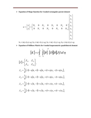
4321
4321
4321
4321
12221121
1121
1222
0000
0000
0000
0000
00
00
1
NNNN
NNNN
NNNN
NNNN
JJJJ
JJ
JJ
J
B
















2
1
00
01
01
)1(
][ 2
v
v
vv
v
E
D
, for plane stress conditions;

















2
21
00
01
01
)21)(1(
][
v
vv
vv
vv
E
D
, for plane strain conditions.
 Equation of element force vector
 







y
xT
e
F
F
NF ][ ;
N – Shape function, Fx – load or force along x direction,
Fy – load or force along y direction.
 Numerical Integration (Gaussian Quadrature)
The Gauss quadrature is one of the numerical integration methods to calculate the
definite integrals. In FEA, this Gauss quadrature method is mostly preferred. In
this method the numerical integration is achieved by the following expression,
 
 

1
1 1
)()(
n
i
ii xfwdxxf
Table gives gauss points for integration from -1 to 1.

33. Number of
Points
n
Location
ix
Corresponding Weights
iw
1 x1 = 0.000 2.000
2
x1, x2 = 895773502691.0
3
1

1.000
3
x1, x3 417745966692.0
5
3

x2=0.000
555555.0
9
5

888888.0
9
8

4 x1, x4= 8611363116.0
x2, x3= 3399810436.0
0.3478548451
0.6521451549
 Problem (I set)
1. Evaluate dx
x
I 

1
1
2
cos

, by applying 3 point Gaussian quadrature and
compare with exact solution.
2. Evaluate dx
x
xeI x







1
1
2
2
1
3 , using one point and two point
Gaussian quadrature. Compare with exact solution.
3. For the isoparametric quadrilateral element shown in figure, determine the
local co –ordinates of the point P which has Cartesian co-ordinates (7, 4).

34. 4. A four noded rectangular element is in figure. Determine (i) Jacobian
matrix, (ii) Strain – Displacement matrix and (iii) Element Stresses. Take
E=2x105
N/mm2
,υ= 0.25, u=[0,0,0.003,0.004,0.006, 0.004,0,0]T
, Ɛ= 0, ɳ=0.
Assume plane stress condition.