Introduction to the Finite Element Method

Introduction to Finite Element Analysis

Mohammad Tawfik

Contents

1 Introduction ....................................................................................................................... 4
2 Numerical Solution of Boundary Value Problems ............................................................. 4
2.1 Objectives .................................................................................................................... 4
2.2 Why Approximate? ..................................................................................................... 4
2.3 Classification of Approximate Solutions of D.E.’s ....................................................... 5
2.4 Basic Concepts............................................................................................................. 5
2.5 General Weighted Residual Method ........................................................................... 6
2.6 Collocation Method..................................................................................................... 9
2.7 The Subdomain Method............................................................................................ 11
2.8 The Galerkin Method ................................................................................................ 13
3 The Finite Element Method ............................................................................................. 17
3.1 Discretization............................................................................................................. 18
3.2 Element Equations .................................................................................................... 18
3.3 Assembling elements’ equations .............................................................................. 21
3.4 Applying Boundary Conditions .................................................................................. 23
3.5 Solving ....................................................................................................................... 23
3.6 Secondary Variables .................................................................................................. 24
3.7 Generalized Procedure for Getting Interpolation Functions .................................... 24
4 Trusses ............................................................................................................................. 29
5 Beams and Frames ........................................................................................................... 33
5.1 Euler-Bernoulli Beam Theory .................................................................................... 33
5.2 Finite Element Trial Functions ................................................................................... 33
5.3 Beam Stiffness Matrix ............................................................................................... 36
6 Two Dimensional Elements.............................................................................................. 38
6.1 A Rectangular Element .............................................................................................. 38
6.2 Assembling 2-D Elements .......................................................................................... 42
7 Stationary Functional Approach ...................................................................................... 46
7.1 Some Definitions ....................................................................................................... 46
7.2 Applications ............................................................................................................... 47
7.2.1 The bar tensile problem ..................................................................................... 47
7.2.2 Beam Bending Problem ..................................................................................... 49
7.3 Plane Elasticity........................................................................................................... 51
7.3.1 Strain-Displacement Relations........................................................................... 52
7.3.2 Strain Energy ...................................................................................................... 52
Introduction 2

7.4 Finite Element Model of Plates in Bending ............................................................... 55
7.4.1 Displacement Function ...................................................................................... 55
7.4.2 Strain-Displacement Relation ............................................................................ 56
7.4.3 Constitutive Relations of Piezoelectric Lamina.................................................. 57
7.4.4 Stiffness and Mass Matrices of the Element ..................................................... 58

Introduction to the finite element method 3

1 Introduction
The finite element method has gained popularity for its simplicity and ability to model
complex domains. The programming of the finite element method has been a task that a lot
of software development firms have taken as its mission to provide the engineering market
with packages that are capable of solving a multitude of problems starting from simple
structure of fluid dynamics problems up to complex problems with coupled fields of
electricity, mechanics of structures, fluid dynamics, and more.

In this course, we will aim at developing the necessary tools for the student to model
physical problems using finite element method as well as programming simple problems of
structure mechanics and some coupled problems. To achieve that aim, simple examples will
be presented and the MATLAB code used to solve the problems will be listed. Further, the
application of symbolic manipulators will be presented using the MATHEMATICA package.

2 Numerical Solution of Boundary Value Problems
Weighted Residual Methods

2.1 Objectives

In this section we will be introduced to the general classification of approximate methods.
One of the approximate methods will receive attention, namely, the weighted residual
method. Derivation of a system of linear equations to approximate the solution of an ODE
will be presented using different techniques as an introduction to the finite element
method.

2.2 Why Approximate?

The question that usually rises in the minds of engineers and students alike is, why do we
study approximate methods? The main answer that should reply to that question is the
ignorance of the humans! Up to this moment, scientists and engineers have been able to
present a vast amount of mathematical models for physical phenomena, unfortunately, a
very small percentage of those models, which are usually in the form of differential
equations, have close form solutions! Thus, the necessity of solving those problems implies
the use of approximate methods to get solutions for some specific problems of certain
interest.

In the modern engineering life, packages that present solutions for problems using digital
computers are everywhere. The understanding of how those packages perform approximate
solutions for a certain physical problem is a necessity for the engineer to be able to use
them. It is always a good idea to be able to predict how the output of the package is going
to be in order to be able to distinguish the right results from errors that may occur due to
bugs in the program or errors in the data given to the program.

On the other hand, an engineer who needs to develop a new technique for the solution of
an advanced, or a new, problem, has to have a good background on how the old problems
were solved.

Introduction 4

2.3 Classification of Approximate Solutions of D.E.’s

Two main families of approximate methods could be identified in the literature. The discrete
coordinate methods and the distributed coordinate methods.

Discrete coordinate methods depend on solving the differential relations at pre-specified
points in the domain. When those points are determined, the differential equation may be
approximately presented in the form of a difference equation. The difference equation
presents a relation, based of the differential equation, between the values of the dependent
variables at different values of the independents variables. When those equations are
solved, the values of the dependent variables are determined at those points giving an
approximation of the distribution of the solution. Examples of the discrete coordinate
methods are finite difference methods and the Runge-Kutta methods. Discrete coordinate
methods are widely used in fluid dynamics and in the solution of initial value problems.

The other family of approximate methods is the distributed coordinate methods. These
methods, generally, are based on approximating the solution of the differential equation
using a summation of functions that satisfy some or all the boundary conditions. Each of the
proposed functions is multiplied by a coefficient, generalized coordinate, that is then
evaluated by a certain technique that identifies different methods from one another. After
the solution of the problem, you will obtain a function that represents, approximately, the
solution of the problem at any point in the domain.

Stationary functional methods are part of the distributed coordinate methods family. These
methods depend on minimizing/maximizing the value of a functional that describes a
certain property of the solution, for example, the total energy of the system. Using the
stationary functional approach, the finite element model of a problem may be obtained. It is
usually much easier to present the relations of different variables using a functional,
especially when the relations are complex as in the case of fluid structure interaction
problems or structure dynamics involving control mechanisms.

The weighted residual methods, on the other hand, work directly on the differential
equations. As the approximate solution is introduced, the differential equation is no more
balanced. Thus, a residue, a form of error, is introduced to the differential equation. The
different weighted residual methods handle the residue in different ways to obtain the
values of the generalized coordinates that satisfy a certain criterion.

2.4 Basic Concepts

A differential equation in the dependent variable f with the independent variable x may be
written in the form:

L f x   g x  or L f x   g x   0


Where L(.) is a linear differential operator and g(x) is the excitation function. The above
equation has to have certain boundary conditions that render the solution unique. If we
select different functions, Ψi, that satisfy all boundary conditions bud do not necessarily
satisfy the differential equation, we may write the approximate solution of f(x) in the form
of:
n
f x    ai i x 
i 1

Where ai are the generalized coordinates, or the unknown coefficients. Applying the
differential operator on the approximate solution, you get:

 n  n
L f x   g x   L  ai i x   g x    ai L i x   g x   0
 i 1  i 1

Note that the right hand side of the above equation is not equal to zero. The non-zero value
of the right hand side is called the reside.
n

 a L x  g x   Rx 
i 1
i i

The admissibility Conditions

The trial functions need to:

• Satisfy all boundary conditions!

• Be differentiable as much as the higher differentiation in the equation

2.5 General Weighted Residual Method

The general weighted residual method is based on integrating the residue multiplied by
weighting functions and then equating the resulting equations by zero. The weighting
functions are any set of functions that are continuous over the domain of the differential
equation. A set functions may be polynomial, sinusoidal, hyperbolic, or any combination of
functions. The number of functions needed should be equal to the unknown generalized
coordinates to produce a set of equations that are solvable in the unknowns. Also, the
weighting functions need to be linearly independent for the equations to be solvable.

Expanding the series of proposed solution functions, we get:

a1L 1 x   a2 L 2 x   ...  an L n x   g x   Rx 

Multiplying by the weighting function and integrating, we get:

Numerical Solution of Boundary Value Problems 6

 n 
 w j x Rx dx 
Domain

Domain
w j x   ai L i x   g x dx  0
 i 1 

 w xRxdx   w xa L x  a L x  ...  a L x  g xdx
Domain
j
Domain
j 1 1 2 2 n n

In matrix form

 k11  ki1  kn1 
     
  
 

k1 j  kij  knj ai     w j x g  x dx 
  Domain
 

     
k1n
  kin  knn 


Where

kij   w x L x dx
Domain
j i

Example Problem

The bar tensile problem is a classical problem that
describes the relation between the axially
distributed loads and the displacement of a bar.
Let’s consider the bar in Figure ‎ .1 with constant
2
modulus of elasticity and cross section area. The
Figure ‎ .1. Sketch of a bar with distributed axial forces
2
force displacement relation is given by:

 2u
EA F 0
x 2

Subject to the boundary conditions

x  0u  0 & x  l  du / dx  0

Now, lets use the approximate solution
n
u x    ai i x 
i 1

Substituting it into the differential equation, we get

n
d 2 i x 
EA ai  F  R x 
i 1 dx 2

Selecting weighting functions, Wi, and applying the method, we get:

l d 2 i x    l 
EA w j x  2
dx ai   F  w j x dx 
0 dx   0 

For the boundary conditions to be satisfied, we need a function that has zero value at x=0
and has a slope equal to zero at the free end. Sinusoidal functions are appropriate for this
hence, using one-term series, we may use:

 x 
 x   Sin 
 2l 

For the weighting function, we may use a polynomial term. The simplest term would be 1.

l  
2
 x   l 
 EA  Sin dx a1   fdx 
 0  2l 
  2l  
 0 

Performing the integration, we get:

     x  
l

 EA   Cos  a1   fl 
  2l  
  2l  0 


When the equation is solved in the unknown coefficient (generalized coordinate), we get:

fl 2l 2 f l2 f
a1    0.637
EA 2l   EA EA

Then, the approximate solution for this problem becomes

l2 f  x 
u x   0.637 Sin 
EA  2l 

Now we may compare the obtained solution with the exact one that may be obtained from
solving the differential equation. The maximum displacement and the maximum strain may
be compared with the exact solution. The maximum displacement is

l2 f
u l   0.637 exact  0.5
EA

And maximum strain is:

u x 0  1.0 exact  1.0
lf
EA


2.6 Collocation Method

The idea behind the collocation method is similar to that behind the buttons of your shirt!
Assume a solution, and then force the residue to be zero at the collocation points.

Rx j   0

The collocation method may be seen as one of the weighted residual family when the
weighting function becomes the delta function. The delta function is one that may be
described as:

 x  x j  1 x  xj
0 x  xj


  x  x F x dx  F x 

j j

Now, if we select a set of points xj inside the domain of the problem, we may write down
the integral of the residue, multiplied by the delta functions, as follows:

Rx j    ai L i x j   F x j   0
n

i 1

Which gives

 k11  ki1  kn1   g x1 
         
  
 kij  knj ai    g x j 
 
k1 j
    
     
 
k1n
  kin  knn 
  g xn 
 

Where

kij  L i x j 



Figure ‎ .2. A sketch of the differences between the exact and approximate solutions
2

Example Problem

Applying this method to the bar tensile problem described before, we get:

n
d 2 i x 
EA ai  F  x   R x 
i 1 dx 2

Evaluating the residue at the collocation points, we get

d 2 i x j 
 F x j   0
n
EA ai
i 1 dx 2

In matrix form

 k11 k 21 ... k n1   a1   F x1 
k  a   
 12 k 22 ... k n 2   2    F x2 
   
         
   F xn 
k1n k 2 n ... k nn  an 
   

Where

d 2 i x 
kij  EA
dx 2 x  x
j

Solve the above system for the “generalized coordinates” ai to get the solution for u(x)

Using Admissible Functions

• For a constant forcing function, F(x)=f

• The strain at the free end of the bar should be zero (slope of displacement is zero).
We may use:

 x 
 x   Sin 
 2l 

Using the function into the DE:

d 2 x     x 
2

EA   EA  Sin 
 2l   2l 
2
dx

A natural selection for the collocation point may be the central point of the bar. Substituting
by the value of x=l/2, we get

f 4 2l 2 f l2 f
a1    0.57
EA 2l  Sin  4  2 EA
2
EA

• Then, the approximate solution for this problem is:

l2 f  x 
u x   0.57 Sin 
EA  2l 

Which gives the maximum displacement to be

l2 f
u l   0.57 exact  0.5
EA

And maximum strain to be:

u x 0  0.9 exact  1.0
lf
EA

2.7 The Subdomain Method

The idea behind the subdomain method is to force the integral of the residue to be equal to
zero on a subinterval of the domain. The method may be also seen as using the unit step
functions as weighting functions. The unit step function may be described by the following
relation:

U x  x j  1 x  xj
0 x  xj
U x  x j   U x  x j 1   1 x j 1  x  x j
0 x  x j or x  x j 1

Hence the integral of the weighted residual method becomes


x j 1

 Rx dx  0
xj

Substituting using the series solution

n x j 1 x j 1

 ai
i 1
 L i x dx 
xj
 g x dx  0
xj

Figure ‎ .3. Sketch of the differences between the exact and approximate solutions
2

For the bar application

d 2 i x 
n
EA ai  F  x   R x 
i 1 dx 2

Performing the integration and equating by zero

d 2 i x 
n x j 1 x j 1

EA ai  dx    F x dx
i 1 xj
dx 2 xj

Which gives the equation in matrix form as

 x j1 d 2 x    x j1
 

EA  i
dx ai     F x dx 
 x j dx 
2
   xj
 


Using Admissible Function

 x 
 x   Sin 
 2l 

The differentiation will give

d 2 x     x 
2

EA   EA  Sin 
 2l   2l 
2
dx

Since we only have one term in the series, we will perform the integral on one subdomain;
i.e. the whole domain

l  
2
 x   l 
 EA  Sin dx a1   fdx 
 0  2l 
  2l  
 0 

Performing the integral

     x  
l

 EA   Cos  a1   fl 
  2l  
  2l  0 


Evaluating the generalized coordinate

fl 2l 2 f l2 f
a1    0.637
EA 2l   EA EA

Then, the approximate solution for this problem is:

l2 f  x 
u x   0.637 Sin 
EA  2l 

Which gives the maximum displacement to be:

l2 f
u l   0.637 exact  0.5
EA

And maximum strain to be:

u x 0  1.0 exact  1.0
lf
EA

2.8 The Galerkin Method

The Galerkin method uses the proposed solution functions as the weighting functions. Thus
the solution procedure will require the selection of one set of functions. That method has
proven very efficient and accurate as a weighted residual method. Many numerical
solutions methods are derived from the Galerkin method. The Galerkin method may be
presented by the following integral


 Rx  x dx  0
Domain
j

When substituting with the series solution, the weighted residual integral will become

n

 a  x L x dx   x g x dx  0
i 1
i j i j
Domain Domain

Applying the Galerkin method to the bar problem, we get

n
d 2 i x 
EA ai   j x  dx    j x F x dx
i 1 Domain
dx 2 Domain

Which in matrix form becomes

 d 2 i x   
 

EA   j x  dx ai     j x F x dx 
Domain 
2
 Domain
 dx 
  

Solve the above system for the “generalized coordinates” ai to get the solution for u(x). Let’s
use the same function as in the previous methods

 x 
 x   Sin 
 2l 

Substituting with the approximate solution:

n
d 2 i x 
EA ai   j x  dx    j x F x dx
i 1 Domain
dx 2 Domain

We have

   x   x     x 
2 l 2 l
 EA  a1  Sin Sin dx   EA  a1  Sin 2   fdx
 2l  0  2l   2l   2l  0  2l 

Which gives

 
2
l 2l
 EA  a1  
 2l  2 

Substituting and solving for the generalized coordinate, we get

f 16l 2 fl 2
a1   0.52
EA  3 EA


In most structure mechanics problems, the differential equation involves second derivative
or higher for the displacement function. When Galerkin method is applied for such
problems, you get the proposed function multiplied by itself or by one of its function family.
This suggests the use of integration by parts. Let’s examine this for the previous example.
Substituting with the approximate solution: (Int. by Parts)

d 2 i x  d x 
l
d j x  d i x 
  j x  2
dx   j x  i   dx
Domain
dx dx 0 Domain dx dx

But the boundary integrals are equal to zero since the functions were already chosen to
satisfy the boundary conditions. Evaluating the integrals will give you the same results.

 
2
l 2l
 EA  a1  
 2l  2 

f 16l 2 fl 2
a1   0.52
EA  3 EA

So, what did we gain by performing the integration by parts?

• The functions are required to be less differentiable

• Not all boundary conditions need to be satisfied

• The matrix became symmetric!

The above gains suggested that the Galerkin method is the best candidate for the derivation
of the finite element model as a weighted residual method.

Homework #1

Figure ‎ .4. A simply supported beam
2

d 4w d 2 w(0) d 2 w(l )
 F ( x) w(0)  w(l )  0 and  0
dx 4 subject to dx 2 dx 2

Exact Solution for this problem is


x 3 13x
w( x)   0  x  1/ 2
12 60
x3 x 2 7 x 3
    1/ 2  x  1
12 4 15 10

• Solve the beam bending problem, for beam displacement, for a simply supported
beam with a load placed at the center of the beam using

– Any weighting function

– Collocation Method

– Subdomain Method

– Galerkin Method

• Use three term Sine series that satisfies all BC’s

• Write a program that produces the results for n-term solution.


3 The Finite Element Method
2 nd order DE’s in 1-D

The finite element method is based on the weighted residual methods presented in the
previous chapter. The main difference of the finite element method is that the proposed
solution functions have generalized coordinates, coefficients, that are equal to the physical
quantity of the unknown variable at some points inside the domain. Hence, the proposed
solution becomes an interpolation function for the values intermediate to those points.

Many physical problems may be approximately presented by 1-D differential equation. Such
a problem will be characterized by having all dependent variables subject in one
independent variable, usually x coordinate, and in initial boundary value problems, the time
will be introduced as another independent variable but the problem will be still considered
a 1-D problem.

Figure ‎ .1 presents a sketch for a general 1-D 2nd order problem. The problem may be
3
considered as one describing the steady state of a heat transfer problem with general
boundary conditions. Different terms are described in the sketch.

nd
Figure ‎ .1. A sketch of the 1-D 2 order problem
3

The problem then may be stated as; solve:

d  du 
  a   cu  f  0
dx  dx 
0 x L

Subject to:

 du 
u 0  u0 ,  a   Q0
 dx  x  L

Now, we will apply the steps of the finite element method to model this problem
approximately.

3.1 Discretization

At the first step of the finite element modeling, we discretize the domain into elements that
all lie inside the domain. Those elements are connected at nodes. At each node, the value of
the dependent variable will be called a degree of freedom.

Figure ‎ .2. Discretization of the domain
3

3.2 Element Equations

Let’s concentrate our attention to a single element. The same DE applies on the element
level; hence, we may follow the procedure for weighted residual methods on the element
level using the boundary conditions as the values of the dependent function at the nodes.
The Finite Element Method 18

d  du 
  a   cu  f  0
dx  dx 
x1  x  x2

Subject to

u x1   u1 , u x2   u2 ,
 du   du 
a   Q1 ,  a   Q2
 dx  x  x1  dx  x  x2

At this step, let’s think about the interpolation of the values of the function over the
element, between the nodes. The most common interpolation function is the polynomial.

Figure ‎ .3. Single 1-D element with the values of the dependent function and the external excitation function
3
determined at the nodes.

Using linear interpolation, we may write

ux   b1 x  b0

Forcing the value of the function to be equal to the given values at the nodes, we get

ux1   u1  b1 x1  b0

ux2   u2  b1 x2  b0

When we solve for the unknown values b0 and b1, and rearranging, we get

 x x   x  x1 
u x    2
 x  x u1   x  x u2
  
 2 1  2 1

Which may be written as

u 
u x    1u1  2u2   1  2  1    x  u e
   
u2 

It may be noticed directly that after rearranging the interpolation function and collecting
terms containing the nodal-values of the dependent variable we get two linear functions


that are used as the proposed solution for the weighted residual method. Note also that the
proposed solution satisfies the essential boundary conditions of the problem; i.e. the values
of the function at the nodes. The sketch of the functions may be seen in Figure ‎ .4
3

Figure ‎ .4. Sketch of the proposed solution functions
3

Note also that the proposed functions do not satisfy the original admissibility conditions
since we are planning to use the Galerkin method as the weighted residual method of
choice.

Assuming constant domain properties a and c may be drawn out of the differentiation in the
differential equation to get

d 2u
a  cu  f  0
dx 2
x1  x  x2

Using the proposed solution obtained in this section and applying the Galerkin method we
get

 d 2 i x  
    a j x  ui  c j x  i x ui  j x  f
 dx  0

Domain 
dx 2 

Note that

 d 2 i x   d x  2
x
d j x  d i x 
    a j x  dx  a j x  i a  dx
Domain 
dx 
2
 dx x1 Domain
dx dx

And

d 1 x  1 d 2 x  1
 , 
dx he dx he

Thus, we may write the integral as


d i x  2
x
d j x  d i x 
ui dx   c j x  i x ui  j x  f dx  0
x x

 a j x 
2 2

 a 
dx x1 x1
dx dx x1

For j=1 we may get the first equation

1 2 1 
2
1
x
a 1  x2  x   x  x  x  x1   x x dx  0
a a   u1  a 2 u2  c
 h   u1  c 2 
 h  h  u2   2
 h f
he he x1  h e
2
he  e   e  e   e  
 

Which gives

 a che   a ch  fh
 
h u1     e u2  e  0
  h 
 e 3   e 6  2

Repeating for using j=2, we get

 a che   a ch  fh
 
 h u1    e u2  e  0
 h 
 e 6   e 3  2

In matrix form

 a  1  1 che 2 1 u1  fhe 1
  
 h  1 1   6 1 2 u   2 1
 e      2  

The above equation is called the element equation.

3.3 Assembling elements’ equations

In the previous section, we obtained the element equation that relates the element degrees
of freedom to the externally applied fields. The element equation may be rewritten in
compact form as

 k1 k2  u1   f1 
k   
 3 k4  u2   f 2 


Now, let’s consider two adjacent elements as in Figure ‎ .5. The element equation for each
3
element may be written as

k12 k2  u12   f12 
2

 2 2  2 
 
 k3 k4  u2   f 22 

k1 k2  u1   f11 
1 1 1

 1 1  1    1 
k3 k4  u2   f 2 

Where the superscript indicates the element number.

Figure ‎ .5. Sketch of two adjacent elements
3
Note that for the continuity of the field values, the value of the function at the right-hand
side of the first element should be equal to that of the left-hand value of the second
element. Hence, we may add the second equation of the first element to the first equation
of the second element to obtain three equations in the three unknown degrees of freedom.

k1
1
k21
0  u1   f1  Q1 
 1 2      
k3 k 4  k12
1
k 2  u2    f 2   Q2 
0
 k32 k 4  u3   f 3
2
  
 Q 
  3

The vector {Q} presents any external fields that are concentrated at the nodes; e.g. Support
reactions in bar problems or fixed temperature in heat transfer problems.

Example

Let us reconsider the bar problem presented in Figure ‎ .1.
2

Divide the bar into N number of elements. The length of each element will be (L/N). Derive
the element equation from the differential equation for constant properties and externally
applied force:

x2
 EA  d j d i 
  h


x1  e 

2 
dx dx
ui  f j  dx  0



The element equation will be obtained as follows

EA  1  1 u1e  fhe 1
 e  
he  1 1  u2  2 1
 

Note that if the integration is evaluated from 0 to h e, where he is the element length, the
same results will be obtained. That is true due to the fact that the bound integration
evaluates the area under the curve, and the area does not change if the axes are
transformed from the origin to x1.

Now, let us consider two–Element bar example,

EA  1  1 u1   f11 
1

  
he  1 1  u1   f 21 
  2

EA  1  1 u12   f12 
 2   
he  1 1  u2   f 22 
 

Assembling the equations as presented above, we obtain

 1  1 0  u1  1  R 
EA   u   fhe 2   0 
 1 2  1  2     
he  u  2 1  0 
 0 1 1  3 
     

Where R is the reaction force at the support of the bar. Note that the external forces
corresponding to the second and third nodes are equal to zero as the problem does not
have any external concentrated forces.

3.4 Applying Boundary Conditions

For the bar with fixed left side and free right side, we may force the value of the left-
displacement to be equal to zero; which is the given boundary condition. The obtained
equation becomes

 1 1 0  0  1  R 
EA   u   fhe 2   0 
 1 2  1  2     
he  u  2 1  0 
 0 1 1  3 
     

Which may be separated into two equations as follows

EA  2  1 u2  fhe 2
   
he  1 1  u3 
  2 1

EA fh
u2  e  R
he 2

Now, we may solve the first equation in the unknown values of the nodal displacements and
then substitute into the second equation to obtain the reaction force.

3.5 Solving

Solving first equation for the displacements, we get

u2  fhe 2 3
   
u3  2 EA 4

Which is the exact value of the displacement that may be obtained if the exact solution was
utilized.

3.6 Secondary Variables

Using the values of the displacements obtained, we may get the value of the reaction force
by substituting into the second equation.

3 fhe fhe
  R
2 2

R  2 fhe

Which is the exact value of the reaction force.

3.7 Generalized Procedure for Getting Interpolation Functions

The need for different types of elements for different structures implied the need for a
generalized methodology to increase the flexibility of the finite element programming. A
large number of proposed trial/interpolation functions is available in the literature, but the
continuous need for development required the development of generalized procedure. In
section ‎ .2, we obtained the element equations for two-node element with linear
3
interpolation functions. Let’s re-derive the equations introducing a more general procedure
then use the same procedure for the derivation of a three-node element.

The interpolation Function

u( x)  a1  a2 x

May be written in matrix form as

ux   H x a

Then, forcing the function to equal the values at the nodes gives

u0  u1  H 0a

ul   u2  H l a

This may be written in matrix form as

u1   H 0  a1  1 0  a1 
          T a
u2   H l  a2  1 l  a2 

Solving for the unknown coefficients, we get


 a1   1 0 u1 
     1 1  
a2   l
 l  2 

u

Or a  T   
1
ue

Substituting into the interpolation function, we get

 
ux   H x T  u e  N x  u e
1
 
Expanding the terms, we find that

 1 0  u   x x  u1 
u x   1 x   1 1  1   1   
 l l  u2   l l  u2 

 

 x x
u ( x)  1  u1  u2
Or  l l

Now, we may write the element equation using the new notation to be

 
l l
EA N x x N x x dx u   N x  fdx  0
e

0 0

Note that

 1   1 2 1
2

l  l      
   dx  1 
1  1
N x x N x x dx    1l  1 1 dx     l  2
l
l 
    1   1 1 
 l l 
2
0 1 li  
    
0

0
 l   l  l  

Which, again, gives the element equation as

EA  1  1 u1e  fhe 1
 e  
he  1 1  u2  2 1
 

Hw 1, x ;
Hwx D Hw, x ;
Hwxx D Hwx, x ;


x 0; Tb1 Hw;
x A; Tb3 Hw;
Clear x ;
TB Tb1, Tb3
TBINV Inverse TB
1, 0 , 1, A
1 1
1, 0 , ,
A A
NN Hw.TBINV
x x
1 ,
A A
A L
Mm Inner Times, Transpose Hw , Hw ;
Mb Integrate Mm, x, 0, A
Mb Transpose TBINV .Mb.TBINV MatrixForm
L
L2 L2 L3
L, , ,
2 2 3
L L
3 6
L L
6 3
CQC Inner Times, Transpose Hwx , Hwx ;
CQC Integrate CQC, x, 0, A
Kb Transpose TBINV .CQC.TBINV MatrixForm
0, 0 , 0, L
1 1
L L
1 1
L L

Let us now try to follow the same procedure to obtain the element matrix for an element
with three nodes. Since we are considering an element with three nodes, we will need a
parabolic interpolation function

Figure ‎ .6. Three-node bar element
3
u( x)  a1  a2 x  a3 x 2

This function may be written in matrix form as

ux   H x a

Using the values of the function at the nodes, we get

u0  u1  H 0a

ul / 2  u2  H l / 2a


ul   u3  H l a

In matrix form

u1   H 0   a1 
    
u2    H l / 2 a2   T a
u   H l   a 
 3   3 

Giving

a  T 1u e 
Finally

 
ux   H x T  u e  N x  u e
1
 
Expanding the function, we get

 x  x2  x  x3   x  x1  x  x3   x  x1  x  x2 
u x   
 x  x  x  x u1   x  x  x  x u2   x  x  x  x u3
       
 1 2  1 3   2 1  2 3   3 1  3 2 

Which may be also written as

 x  l / 2  x  l   x  x  l   x  x  l / 2 
u x     u1    u2    u3
 l / 2  l   l / 2  l / 2   l  l / 2 

Where “l” is the element length. The proposed solution functions may be plot as in
Figure ‎ .7. Note that each of the three functions is equal to one at its corresponding point
3
and zero at the other two points.

Figure ‎ .7. Plot of the proposed solution functions for A 3-node element
3


Hw 1, x, x x ;
Hwx D Hw, x ;
Hwxx D Hwx, x ;

x 0; Tb1 Hw;
x A; Tb3 Hw;
x A 2; Tb2 Hw;
Clear x ;
TB Tb1, Tb2, Tb3
TBINV Inverse TB
A A2 2
1, 0, 0 , 1, , , 1, A, A
2 4
3 4 1 2 4 2
1, 0, 0 , , , , , ,
A A A A2 A2 A2
NN Hw.TBINV
3x 2 x2 4x 4 x2 x 2 x2
1 , ,
A A2 A A2 A A2
A L
Mm Inner Times, Transpose Hw , Hw ;
Mb Integrate Mm, x, 0, A
Mb Transpose TBINV .Mb.TBINV MatrixForm
L
L2 L3 L2 L3 L4 L3 L4 L5
L, , , , , , , ,
2 3 2 3 4 3 4 5
2L L L
15 15 30
L 8L L
15 15 15
L L 2L
30 15 15
CQC Inner Times, Transpose Hwx , Hwx ;
CQC Integrate CQC, x, 0, A
Kb Transpose TBINV .CQC.TBINV MatrixForm
2 2 4 L3
0, 0, 0 , 0, L, L , 0, L ,
3
7 8 1
3L 3L 3L
8 16 8
3L 3L 3L
1 8 7
3L 3L 3L


4 Trusses
A truss is a set of bars that are connected at frictionless joints. The bar does not undergo
deformations normal to its axis but when another one that is connected to and is not coaxial
with it deforms it rotates around its axis. Since the truss is mainly a set ob bars that
generally oriented in the plane and connected to one another, then we have to consider its
general motion. Now, the problem lies in the transformation of the local displacements of
the bar, which are always in the direction of the bar, to the global degrees of freedom that
are generally oriented in the plain.

Figure ‎ .1. A truss element generally oriented in the plane (a) Displacements and forces in the bar local coordinate (b)
4
Resolution of the displacements and forces in the global coordinates
Consider the truss element presented in Figure ‎ .1. The force-displacement equations in the
4
local coordinates of the element may be presented by

1 0 1 0  u1   F 1 
    
EA  0 0 0 0  v1   0 
    
h  1 0 1 0 u 2   F 2 
 
0 0 0 0  v 2   0 
   

From the geometry, the local and global coordinates may be related using the relation

u1   Cos   Sin   0 0  u1 
   Sin   Cos    
 v1   0 0  v1 
 
  
u2   0 0 Cos   Sin    u2 
 
v 2 
  LocalDOF  0 0  Sin   Cos   v2 Transforme
  DOF d

Or

 Local DOF  T Transforme
DOF
d



Where  and  are the displacements in local and global coordinates respectively and
the transformation matrix is

 Cos   Sin   0 0 
 Sin   Cos   0 0 
T    
 0 0 Cos   Sin   
 
 0 0  Sin   Cos  

The Equation of Motion Becomes

K T   F
Transforming the forces:

T 1K T   T 1F 
Note that

T 1  T T
Finally

K   F 
where

K   T T K T 
Where

1 0  1 0
 0 0 0
 
K 
EA  0
h  1 0 1 0

 
0 0 0 0

Element Stiffness Matrix in Global Coordinates becomes

Cos   Sin   0 0  1 0  1 0  Cos   Sin   0 0 
 Sin   Cos  0 0  0   Sin   Cos 
0 0 0  0 0 
K   EA   
h  0 0 Cos   Sin    1 0 1 0  0 0 Cos   Sin   
   
 0 0 Sin   Cos     0 0 0 0  0 0  Sin   Cos 

Or

Trusses 30

 
 Cos   Sin 2   Cos 2    Sin 2 
2 1 1
2 2
 1 
 Sin 2  Sin    Sin 2   Sin 2   
2 1
K   EA  2 2 
h   Cos 2    1 Sin 2  Cos  
2 1
Sin 2  
 2 2 
 1 
 Sin 2   Sin   Sin 2  Sin 2   
2 1
 2 2 

Example

Use the finite element analysis to find the displacements of node C and the stresses in each
element.

Figure ‎ .2. The truss of the example
4
The stiffness matrix in global coordinates of each of the truss elements may be written as

1 0  1 0 0 0 0 0
 0 0 0  0  1
 
K1 
EA  0
L  1 0 1 0
  
K2 
EA 0 1
L 0 0 0 0

   
0 0 0 0 0  1 0 1

 0.3536 0.3536  0.3536  0.3536
 0.3536  0.3536  0.3536
 
K3 
EA  0.3536
L  0.3536  0.3536 0.3536

0.3536 
 
 0.3536  0.3536 0.3536 0.3536 

Assembling the matrices into the global stiffness matrix, we get

 1.3536 0.3536  1 0  0.3536  0.3536
 0.3536 0.3536 0 0  0.3536  0.3536
 
EA   1 0 1 0 0 0 
K    
L  0 0 0 1 0 1 
 0.3536  0.3536 0 0 0.3536 0.3536 
 
 0.3536  0.3536 0  1 0.3536
 1.3536 



Similarly, the force vector is obtained as

 F1x   F1x 
F   
 1 y   F1 y 
F   F 
F    2 x    2 x 
   
 F2 y   F2 y 
 F3 x   P 
   
 F3 y   2 P 
   

The boundary conditions of the truss are

U1  V1  U 2  V2  0

Removing the corresponding rows and columns, we get

EA 0.3536 0.3536 U 3   P 
  
L 0.3536 1.3536  V3   2 P 
 

Solving for the displacements, we get

PL 3PL
U 3  5.828 , V3  
EA EA

Using the secondary equations to get the reaction forces, we get

F1x   P, F1 y   P, F2 x  0, F2 y  3P

Performing post-computation, we get
e e
P1 P 2
 
e

Ae Ae

 P1  Ae Ee  1  1 u1 
 
e e
 
 e   e
P 2 
  L  1 1  u 2 
  

u1   Cos   Sin   0 0  u1 
    
 v1   Sin   Cos   0 0  v1 
 
 
u2   0 0 Cos   Sin    u2 
v 2   0 
 Sin   Cos   v2 
   0  

Finally

3P P
 (1)  0,  ( 2)   ,  ( 3)  2
A A

Trusses 32

5 Beams and Frames
Beams are the most-used structural elements. Many real structures may be approximated
as beam elements. Two main beam theories; Euler-Bernoulli beam theory and Timoshenko
beam theory. In this chapter, we will be focusing out attention to the Euler-Bernoulli beam
theory.

5.1 Euler-Bernoulli Beam Theory

The main assumption in the Euler-Bernoulli beam theory is that the beam’s thickness is too
small compared to the beam length. That assumption resulted in that the sheer deformation
of the beam may be neglected without much error in the analysis. The equation governing
the deformation of and E-B beam under transverse loading may be written as follows

d2  d 2w 
 EI x  2   F ( x)
dx 2 
 dx  

Subject to any combination of the following boundary conditions. At x=0

d 3w0
w0  w0 or EI 0  P0
dx3

Indicating that either the deflection or the sheer force is specified

dw0 d 2 w0
 w'0 or EI 0  M0
dx dx 2

Indicating that either the slope or the bending moment is specified. At x=l

d 3wl 
wl   wl or EI l   Pl
dx3

Indicating that either the deflection or the sheer force is specified

dwl  d 2 wl 
 w'l or EI l   Ml
dx dx 2

Indicating that either the slope or the bending moment is specified.

Where w is the transverse deflection of the beam, E is the modulus of elasticity, I is the
second moment of area, and F is the transverse load in the positive direction of w.

5.2 Finite Element Trial Functions
The finite element model for the EB beam will depend on the knowledge of four boundary
conditions, namely, the deflections and slopes at each node of the element (see Figure ‎ .1).
5


That will require the use of a third order polynomial to interpolate the deflection function in
the element.

w( x)  a1  a2 x  a3 x 2  a4 x3

Figure ‎ .1. Sketch of a beam element
5
Using the same procedure adopted for the bar element, we get

wx   H x a

Enforcing the boundary conditions

w0  w1  H 0a

wl   w2  H l a

w' 0  w'1  H x 0a

w' l   w'2  H x l a

In matrix form

 w1   H 0   a1 
 w'   H 0 a 
 1   x  2 
     T a
 w2   H l   a3 
w'2   H x l   a4 
    

Or

 w1  1 0 00   a1 
 w'  0 1 0 0  a 2 
 1   
  3  
 w2  1 l  a3 
2
l l
w'2  0
  

1 2l 3l 2  a4 
 

Solving

Beams and Frames 34

 1 0 0 0
 a1    w1 
a   0 1 0 0  
 2 3 2 3  1  w'1 
  2  
a3   l l l2 l   w2 
a 4   2 1 2 1  w' 
   3  2
l l2 l3 l2 


Which gives wx   H x a  N x  e  Where
u

 3x 2 2 x 3 
1  2  3 
 l l 
x 2 x 2 x3 
 3
 l 
 N  x   N  x    l
T
2 3 
 3x  2 x 
 l2 l3 
 x 2
x3 
   2 
 l l 

Plotting the four functions, we get the graph in Figure ‎ .2. Notice that N1 and N3 functions
5
are equal to one at x=0 and x=1 respectively while equal to zero at x=1 and x=0 respectively
which can also be related to the fact that N1 and N3 correspond to w1 and w2 respectively.
Similarly, N2 and N4 have zero slopes at x=l and x=0 respectively and are corresponding to
w’1 and w’2 respectively. Now we may write down the displacement function in terms of
the nodal displacements as follows

 
wx   H x a  H x T  we  N x  we
1
 
Or
4
wx    N i x wi
i 1

1
N1 N3
0.8
0.6
0.4
N(x)

0.2 N2
0
-0.2 0 0.2 0.4 0.6 0.8 N4 1

-0.4
X

Figure ‎ .2. A plot of the beam interpolation functions.
5

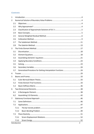
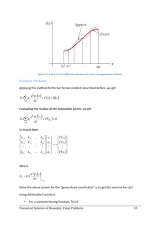
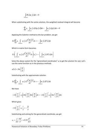
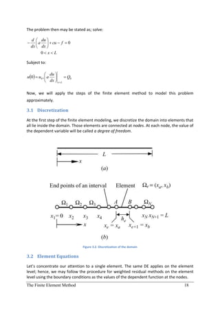
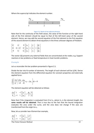
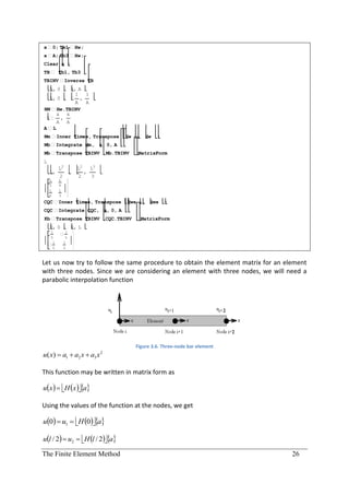
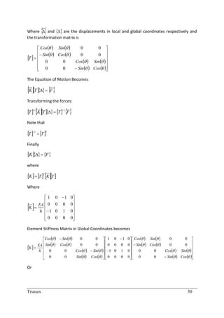
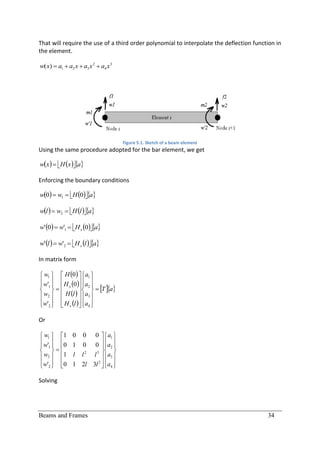
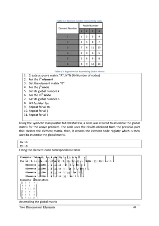
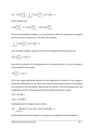
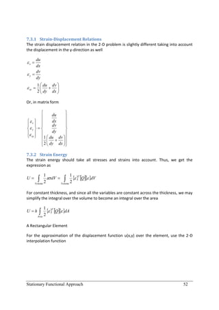
The symbolic manipulator MATHEMATICA may be used to derive the trial functions N(x) as
presented below

In[2]:= Hw 1, x, x x, x x x ;
Hwx D Hw, x ;
Hwxx D Hwx, x ;

In[5]:= x 0; Tb1 Hw; Tb2 Hwx;
x L; Tb3 Hw; Tb4 Hwx;

Clear x ;
TB Tb1, Tb2, Tb3, Tb4
TBINV Inverse TB

Out[8]= 1, 0, 0, 0 , 0, 1, 0, 0 , 1, L, L 2 , L 3 , 0, 1, 2 L, 3 L 2

3 2 3 1 2 1 2 1
Out[9]= 1, 0, 0, 0 , 0, 1, 0, 0 , , , , , , , ,
2 2 3 2 3
L L L L L L L L2

In[10]:= NN Hw.TBINV

3 x2 2 x3 2 x2 x3 3 x2 2 x3 x2 x3
Out[10]= 1 , x , ,
2 3 2 2 3
L L L L L L L L2

In[11]:= Simplify NN

L x 2 L 2x L x 2x 3L 2 x x2 x2 L x
Out[11]= , , ,
3 2 3
L L L L2

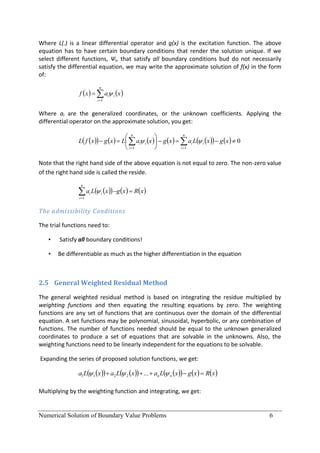
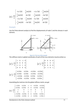
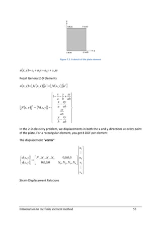
5.3 Beam Stiffness Matrix
Recall that the governing equation is

d2  d 2w 
 EI x  2   F ( x)
dx 2 
 dx  

Substituting with the series solution obtained in the previous section
4
wx    N i x wi
i 1

The governing equation becomes

4
d2  d 2N 
 dx 2  EI x  2 i wi   F ( x)  R( x)

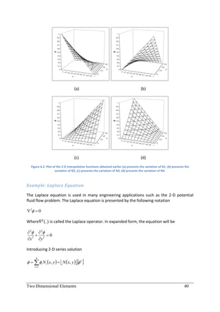
i 1  dx 

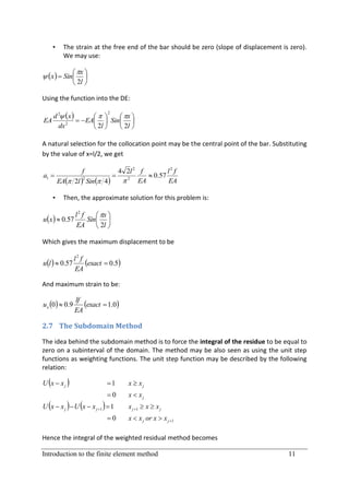
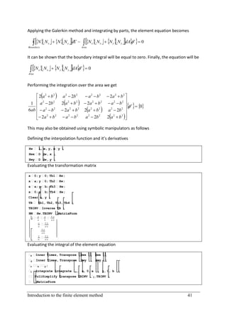
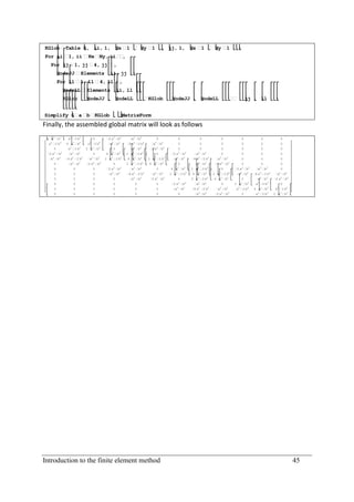
Applying Galerkin method:

Beams and Frames 36

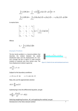
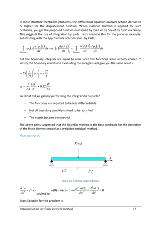
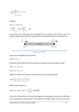
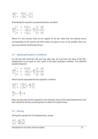
le le
 4 d2  d 2N  
 R( x) N j dx     2  EI x  2 i wi   F ( x)  N j dx
 dx   
0 0  i 1  dx  

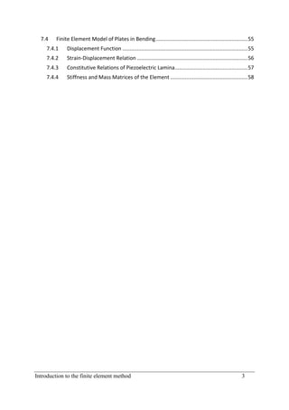
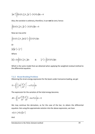
Using integration by parts, twice, we get:

le
 4  2
d 2N j  
   EI x  d N i wi   F ( x) N j dx  0
  i1  dx 2 dx 2  
0   

In matrix form
le le

 EI x N N dxw   F ( x)N xx dx
e
xx xx
0 0

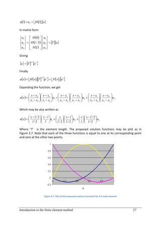
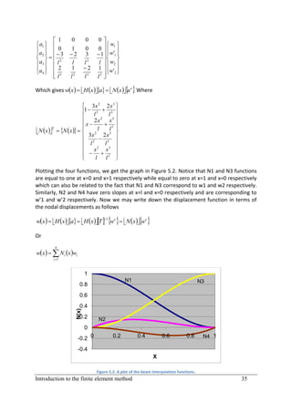
Using MATHEMATICA, we get

In[2]:= Hw 1, x, x x, x x x ;
Hwx D Hw, x ;
Hwxx D Hwx, x ;

In[5]:= x 0; Tb1 Hw; Tb2 Hwx;
x L; Tb3 Hw; Tb4 Hwx;

Clear x ;
TB Tb1, Tb2, Tb3, Tb4
TBINV Inverse TB

Out[8]= 1, 0, 0, 0 , 0, 1, 0, 0 , 1, L, L 2 , L 3 , 0, 1, 2 L, 3 L 2

3 2 3 1 2 1 2 1
Out[9]= 1, 0, 0, 0 , 0, 1, 0, 0 , , , , , , , ,
2 2 3 2 3
L L L L L L L L2

In[10]:= NN Hw.TBINV

3 x2 2 x3 2 x2 x3 3 x2 2 x3 x2 x3
Out[10]= 1 , x , ,
L2 L3 L L2 L2 L3 L L2

In[11]:= Simplify NN

L x 2 L 2x L x 2x 3L 2 x x2 x2 L x
Out[11]= , , ,
3 2 3 2
L L L L

Giving the stiffness matrix to be


6 Two Dimensional Elements
More complicated and realistic problems can not be approximated by one dimensional
elements. Problems such as 2-D fluid flow, heat conduction, plate bending, ocean dynamics,
and others need a two dimensional element to be used. We will focus in this chapter on 2-D
rectangular elements with 1 DOF per node. Later, we will introduce more general elements.

6.1 A Rectangular Element
For the rectangular element presented in Figure ‎ .1, the four nodes have the coordinates
6
shown relative to local coordinate system sat has its origin at point 1. For the problem
where one dependent variable is being investigated, we may interpolate that function using

Figure ‎ .1. Sketch of a 2-D rectangular element.
6
f x, y   a1  a2 x  a3 y  a4 xy

Which is a 2-D function composed of two linear terms multiplied by each other. The
function may be presented in the general form

f x, y   H x, y a

Now, relating the generalized coordinated to the degrees of freedom at each node, we get

f 0,0  f1  H 0,0a

f a,0  f 2  H 0, a a

f a, b  f 3  H a, ba

f 0, b  f 4  H 0, ba

In matrix form

Two Dimensional Elements 38

 f1   H 0,0  a1 
 f   H a,0 a 
 2    2   T a
   
 f 3   H a, b  a3 
 f 4   H 0b   a4 
    

Or

 f1  1 0 0 0   a1 
 f  1 a 0 0  a 2 
 2   
   
 f 3  1 a b ab a3 
 f 4  1
  

0 b 0  a 4 
 

Inverting the transformation matrix, we get

1 0 0 0
 a1    1 1
0

0   f1 
a   a a f 
 2   1 1  2 
  0 0  f 
a3   b b  3 
a 4   1
  1 1  1  f 4 
 
 ab
 ab ab ab 


Giving the interpolation function as

 
f x, y   H x, y a  N x, y  f e

Where

 x y xy 
1  a  b  ab 
 x xy 
  
 
 N  x, y   N  x, y    a ab
T
xy 
 
 ab 
 y xy 
 b  ab
 


Figure ‎ .2 presents the variation of the functions N1 through N4 in the 2-D domain. Note
6
that each of the function is equal to one at the node that corresponds to it while equals zero
at the three other nodes.


1 1

0.9 0.9

0.8 0.8

0.7 0.7

0.6 0.6
N1 0.5 N2 0.5

0.4 0.4

0.3 0.3

0.2 0.2
0.9 0.9
0.1 0.1
0.6 0.6
0 y 0 y
0.3 0.3
0 0.1 0 0.1
0.2 0.3 0.2 0.3
0.4 0.5 0 0.4 0.5 0
0.6 0.7 0.6 0.7
0.8 0.9 0.8 0.9
x 1 x 1

(a) (b)

1 1

0.9 0.9

0.8 0.8

0.7 0.7

0.6 0.6
N3 0.5 N4 0.5

0.4 0.4

0.3 0.3

0.2 0.2
0.9 0.9
0.1 0.1
0.6 0.6
0 y 0 y
0.3 0.3
0 0.1 0 0.1
0.2 0.3 0.2 0.3
0.4 0.5 0 0.4 0.5 0
0.6 0.7 0.6 0.7
0.8 0.9 0.8 0.9
x 1 x 1

(c) (d)
Figure ‎ .2. Plot of the 2-D interpolation functions obtained earlier (a) presents the variation of N1, (b) presents the
6
variation of N2, (c) presents the variation of N3, (d) presents the variation of N4.

Example: Laplace Equation

The Laplace equation is used in many engineering applications such as the 2-D potential
fluid flow problem. The Laplace equation is presented by the following notation

 2  0

Where is called the Laplace operator. In expanded form, the equation will be

 2  2
 0
x 2 y 2

Introducing 2-D series solution

   i N i x, y   N x, y  e 
4

i 1


Applying the Galerkin method and integrating by parts, the element equation becomes

 N N   N N d   N N   N N dA  0
e
x y x x y y
Boundary Area

It can be shown that the boundary integral will be equal to zero. Finally, the equation will be

 N N   N N dA  0
e
x x y y
Area

Performing the integration over the area we get


 2 a 2  b2  a 2  2b 2  a 2  b2  2a 2  b 2 

1  a 2  2b 2 
2 a 2  b2   2a 2  b 2  a2  b2  e

 
  0
6ab   a 2  b 2

 2a 2  b 2 
2 a2  b2  a 2  2b 2 

  2a  b

2 2
 a 2  b2 a 2  2b 2 
2 a 2  b2   
This may also be obtained using symbolic manipulators as follows

Defining the interpolation function and it’s derivatives

Hw 1, x, y, x y ;
Hwx D Hw, x ;
Hwy D Hw, y ;
Evaluating the transformation matrix

x 0; y 0; Tb1 Hw;
x a; y 0; Tb2 Hw;
x a; y b; Tb3 Hw;
x 0; y b; Tb4 Hw;
Clear x, y ;
TB Tb1, Tb2, Tb3, Tb4 ;
TBINV Inverse TB ;
NN Hw.TBINV MatrixForm
x y xy
1
a b ab
x xy
a ab
xy
ab
y xy
b ab

Evaluating the integral of the element equation

x Inner Times, Transpose Hwx , Hwx ;
y Inner Times, Transpose Hwy , Hwy ;
o x y;

1 Integrate Integrate o, x, 0, a , y, 0, b ;
FullSimplify Transpose TBINV . 1.TBINV ;
MatrixForm


a2 b2 a b a2 b2 a b
3ab 6b 3a 6ab 3b 6a
a b a2 b2 a b a2 b2
6b 3a 3ab 3b 6a 6ab
a2 b2 a b a2 b2 a b
6ab 3b 6a 3ab 6b 3a
a b a2 b2 a b a2 b2
3b 6a 6ab 6b 3a 3ab

6.2 Assembling 2-D Elements

The Logistic Problem!

In the 2-D problems, the numbering scheme, usually, is not as straight forward as the 1-D
problem. For example, in 1-D problem as that shown in Figure ‎ .3, we can easily relate the
6
nodes’ numbers to the elements’ numbers. Although the finite element method does not
mandate the numbering scheme, it is usually more practical to use the simplest scheme.

Figure ‎ .3. 1-D elements’ connectivity and nummbering
6

Figure ‎ .4. Example of 2-D connectivity and numbering scheme
6

Table ‎ .1. Relation between local and global node numbering for element number 5
6
Local Node Global Node
Number Number
1 5
2 6
3 9
4 8

In a 2-D problem, such as that shown in Figure ‎ .4, the node and element numbering
6
becomes more complicated than the 1-D problem, although, an easy relation may still be


obtained between the nodes’ and the elements’ numbering it is not advised to keep on
applying this relation inside the program. Rather, a register should be filled in which each
number is related to the nodes to which it is connected. Table ‎ .1 shows the register entry
6
for element number 5. The register entry contains the local node number and the
corresponding global node number. From the register, it is easy to determine which entry in
the global matrix each of the element matrix entries should be added to. Figure ‎ .5 shows,
6
graphically, the locations of in the global matrix to which the element matrix entries should
be added.

1 2 3 4 5 6 7 8 9 10 11 12
1
2
3
4
5 1,1 1,2 1,4 1,3
6 2,1 2,2 2,4 2,3
7
8 4,1 4,2 4,4 4,3
9 3,1 3,2 3,4 3,3
10
11
12
Figure ‎ .5. Entries of the global matrix corresponding to each entry of the element matrix of element number 5.
6

The procedure presented above for the element number 5 is now going to be generalized
for the rest of the elements. Table ‎ .2 presents the local-to-global correspondence node
6
numbering for the 2-D problem presented in Figure ‎ .4.
6
Now we need to apply the procedure used for element number 5, explained above, to the rest of the elements.
Table ‎ .3 presents an algorithm that may be used for assembling the global matrix for a 2-D
6
problem with a single degree of freedom per node. The algorithm is based on scanning the
nodes of each element, reading their corresponding global number and adding the local
matrix entry to the corresponding global matrix entry. Thus, two loops on the elements’
nodes are used together with the main elements’ loop.


Table ‎ .2. Element number connectivity table.
6
Node Number
Element Number
1 2 3 4

1 1 2 5 4

2 4 5 8 7

3 7 8 11 10

4 2 3 6 5

5 5 6 9 8

6 8 9 12 11

Table ‎ .3. Algorithm for Assembling Global Matrix
6
1. Create a square matrix “A”; N*N (N=Number of nodes)
2. For the ith element
3. Get the element matrix “B”
4. For the jth node
5. Get its global number k
6. For the mth node
7. Get its global number n
8. Let Akn=Akn+Bjm
9. Repeat for all m
10. Repeat for all j
11. Repeat for all i

Using the symbolic manipulator MATHEMATICA, a code was created to assemble the global
matrix for the above problem. The code uses the results obtained from the previous part
that creates the element matrix, then, it creates the element-node registry which is then
used to assemble the global matrix.

Nx 2;
Ny 3;
Filling the element-node correspondence table

Elements Table 0, ii, 1, Nx Ny , jj, 1, 4 ;
For ii 1, ii Nx, ii , For jj 1, jj Ny, jj , ElNm jj Ny ii 1 ;
Elements ElNm , 1 ii jj 1 Nx 1 ;
Elements ElNm , 2 ii 1 jj 1 Nx 1 ;
Elements ElNm , 3 ii 1 jj Nx 1 ;
Elements ElNm , 4 ii jj Nx 1 ; ;
Elements MatrixForm
1 2 5 4
4 5 8 7
7 8 11 10
2 3 6 5
5 6 9 8
8 9 12 11
Assembling the global matrix

KGlob Table 0, ii, 1, Nx 1 Ny 1 , jj, 1, Nx 1 Ny 1 ;
For ii 1, ii Nx Ny, ii ,
For jj 1, jj 4, jj ,
NodeJJ Elements ii, jj ;
For ll 1, ll 4, ll ,
NodeLL Elements ii, ll ;
KGlob NodeJJ , NodeLL KGlob NodeJJ , NodeLL jj , ll ;
;
Simplify 6 a b KGlob MatrixForm
Finally, the assembled global matrix will look as follows
2 a2 b2 a2 2 b2 0 2 a2 b2 a2 b2 0 0 0 0 0 0 0
a2 2 b2 4 a2 b2 a2 2 b2 a2 b2 4 a2 2 b2 a2 b2 0 0 0 0 0 0
0 a2 2 b2 2 a2 b2 0 a2 b2 2 a2 b2 0 0 0 0 0 0
2 a2 b2 a2 b2 0 4 a2 b2 2 a2 2 b2 0 2 a2 b2 a2 b2 0 0 0 0
a2 b2 4 a2 2 b2 a2 b2 2 a2 2 b2 8 a2 b2 2 a2 2 b2 a2 b2 4 a2 2 b2 a2 b2 0 0 0
0 a2 b2 2 a2 b2 0 2 a2 2 b2 4 a2 b2 0 a2 b2 2 a2 b2 0 0 0
0 0 0 2 a2 b2 a2 b2 0 4 a2 b2 2 a2 2 b2 0 2 a2 b2 a2 b2 0
2 2 2 2 2 2 2 2 2 2 2 2 2 2 2 2 2
0 0 0 a b 4a 2b a b 2 a 2b 8 a b 2 a 2b a b 4a 2b a b2
2 2 2 2 2 2 2 2 2 2
0 0 0 0 a b 2a b 0 2 a 2b 4 a b 0 a b 2 a2 b2
0 0 0 0 0 0 2 a2 b2 a2 b2 0 2 a2 b2 a2 2 b2 0
0 0 0 0 0 0 a2 b2 4 a2 2 b2 a2 b2 a2 2 b2 4 a2 b2 a2 2 b2
0 0 0 0 0 0 0 a2 b2 2 a2 b2 0 a2 2 b2 2 a2 b2


7 Stationary Functional Approach
In this section, the stationary functional approach will be presented as a method by which
the finite element model may be derived. The approach will depend on some definitions
that are presented in section ‎ .1 then some applications will be presented in the following
7
sections.

7.1 Some Definitions

A Functional: Simple Definition

A functional is a “function of functions” that produces a real/complex number. The
functional is presented in the form of a bound integral which, when evaluated, produces a
real number. In mechanics problems, usually, the functional used is the total energy
functional which contains the potential energy, the kinetic energy, and the externally work
done on the system. A functional may be presented in the form

I  f1 x1 ,..., xn ,..., f m x1 ,..., xn    G f x ,..., x ,..., f x ,..., x dx ...dx
1 1 n m 1 n 1 n
Domain

Variation: Another simple definition

Variation of a functional is the “differentiation” of the functional with respect to one or
more of its entries (functions). Note that the Variation of the functional with respect to the
independent variables is always equal to zero.

 dG 
I  f1 , f 2 ,..., f m  
dG dG
  df1

Domain
f1 
df 2
f 2  ... 
df m
f m dx1...dxn



Stress-Strain Relation

Stresses in structures are related to the strains through “constitutive relations”. The main
components of the constitutive relations is the modulus of elasticity, Hook’s constants. For
1-D structures, we may write

  E

Strain Displacement Relations

The strain is usually related to the displacement fields in structure mechanics problems. The
relation may be obtained from the theory of elasticity or an approximate theory such as the
Euler-Bernoulli beam theory. For 1-D elasticity problems, the strain displacement relations
are usually simple ones such as the case of a bar, where the relation is defined as

du
x 
dx

Where u is the axial displacement of the bar. Meanwhile, the strain displacement relation
for an Euler-Bernoulli beam is given by
Stationary Functional Approach 46

d 2w
 x  z
dx 2

Where w is the transverse deflection of the beam and z is the location above the neutral
axis. Other relations exist for different theories, but they will be mentioned in their
respective places.

Strain Energy

Strain energy is the amount of mechanical energy stored in a structure, potential energy,
due to the deflection of the structure. An expression for the strain energy may be given by

1
U 
Volume
2
 dV

Where U is the strain energy. The concept here is defined for linear elastic structures, but
may be used for nonlinear material properties as well as dissipative material properties with
minor constraints.

7.2 Applications

In the following sections, we will present the application of the concepts of variation and
strain energy to obtain the finite element model as well as demonstrate that the
presentation is equivalent to the more commonly used differential equation presentation.

7.2.1 The bar tensile problem
The total energy of the elastic structure is given as the difference between the strain energy
and the work done by the externally applied forces. An expression for the total energy for a
bar, may be given by the following integral

 1  u  2 
    EA   u.F x dx
 2  x  
BarLength 

For equilibrium, the total energy needs to be at a minimum value, that is to say, its variation
is zero (note the analogy with the minimum of a function in one dimension where the
extreme points are found when the derivative is equal to zero. Obtaining the variation of
the total energy, we get

  u  u  
    EA
    u.F x dx  0

BarLength  x  x  

Now, let us perform integration by parts, we get


 
l
 u    2u 
  EAu      EAu 2   u.F x dx  0
 x 
 x  0 BarLength 
  

Which indicates that
l
 u   u   u 
EAu   0  EAu   0 & EAu 
 x  0  x  x  0  x  x  l

These are the boundary conditions; i.e. at any boundary, either the displacement is equal to
zero or the strain is equal to zero. The other term becomes

   2u  
   EAu 2   u.F x dx  0
 x  
BarLength   

Since the above integral is equal to zero, then the integrand should be equal to zero

   2u  
u EA 2   F x   0
  x  
   

And, since the variation of the displacement is an arbitrary function, it can not be equal to
zero everywhere which yields

  2u 
EA 2   F x   0
 x 
 

This is the original differential equation for the displacement function of a bar subject to
distributed loading along its axis. Now, if we select the approximate solution of the problem
and substitute it into the equation representing the variation of the total energy, above, and
handling the variation of the displacement as the weighting functions, we get

 
ux   N x  u e

ux   N x  u e 


Substituting into the energy variation relation:

   EAu  N N u  u  N F xdx  0
e T e e T
x x
ElementLength

But the nodal values of the function or its variation are independent of the integration


u   EAN N u  N F xdx  0
l
e T e
x x
0

Also, the variation is arbitrary, therefore, it can not be zero; hence:

 EAN N u  N F x dx  0
l
e
x x
0

Now we may write

 EAN x N x dxu   N F x dx
l l
e

0 0

Or

k u e  f e 
Where

f   N F xdx
l l
k   EA N x N x dx & e

0 0

Which is the same model that we obtained when applying the weighted residual method to
the differential equation.

7.2.2 Beam Bending Problem
Obtaining the strain energy expression for the beam under transverse loading, we get

 1  d 2 w 2
l 
    EI  2   w.F x dx
0
 2  dx 
  


The expression for the variation of the total energy becomes

 d 2w d 2 w
l

    EI
 2 2
 w.F x dx  0

0 
dx dx

We may continue the derivation, as for the case of the bar, to obtain the differential
equation. But using the approximate solution into the above expression, we have

wx   N x  we  
And


wx   N x  we 


Which gives

 
   EI  we  N xx N xx we   we  N F x  dx  0
l
 
T T

0

Using the same procedure as for the bar example above, we get

k we  f e 
Where

f   N F xdx
l l
k    EI N xx N xx dx & e

0 0

Which is, again, the same model as the one obtained using the weighted residual methods.


7.3 Plane Elasticity

Now, we have enough background to extend our study to cover the plain elasticity problem.
In this problem we are only concerned with the thin structures, such as thin plates, that are
subjected to in-plane loading. In such a problem, the strain components we are concerned
with become the axial strains in the plane of the plate and the shear strain component
associated with them. All variables are assumed to constant across the thickness.

Figure ‎ .1. A sketch presenting a plain element with the stresses applied on it.
7

The above described stresses and strain are related through the following relations

 x  D x  D y
 y  D x  D y
 xy  2G xy

Where

E
D
1  2
E
G
21  

In matrix form

 x   D D 0    x 
    
 y   D D 0    y 
   0 0 2G   xy 
 xy    

Or

   Q 

7.3.1 Strain-Displacement Relations
The strain displacement relation in the 2-D problem is slightly different taking into account
the displacement in the y-direction as well

du
x 
dx
dv
y 
dy
1  du dv 
 xy    
2  dy dx 
 

Or, in matrix form

 
 du 
x   dx 
   dv 
 y    
   dy 
 xy   1  du dv 
 2  dy  dx 
 
  

7.3.2 Strain Energy
The strain energy should take all stresses and strains into account. Thus, we get the
expression as

 dV    T Q dV
1 1
U 
Volume
2 Volume
2

For constant thickness, and since all the variables are constant across the thickness, we may
simplify the integral over the volume to become an integral over the area

 2   Q dA
1
U h
T

Area

A Rectangular Element

For the approximation of the displacement function u(x,y) over the element, use the 2-D
interpolation function


Figure ‎ .2. A sketch of the plate element
7

ux, y   a1  a2 x  a3 y  a4 xy

Recall General 2-D Elements

 
ux, y   H x, y a  N x, y  u e

 x y xy 
1  a  b  ab 
 x xy 
  
 
N x, y   N x, y    a ab
T
xy 
 
 ab 
 y xy 
 b  ab
 


In the 2-D elasticity problem, we displacements in both the x and y-directions at every point
of the plate. For a rectangular element, you get 8 DOF per element

The displacement “vector”

u1 

 
u  x, y   N1 , N 2 , N 3 , N 4 0,0,0,0  
 u4 
   v 
vx, y   0,0,0,0 N1 , N 2 , N 3 , N 4   1 

 
 v4 
 

Strain-Displacement Relations


 du  u1 
  
  x   dx   N1x , N 2 x , N 3 x , N 4 x 0,0,0,0  
   dv    
 u 
 y     0,0,0,0 N1 y , N 2 y , N 3 y , N 4 y   4 
   dy   N , N , N , N v
 xy   du dv   1 y 2 y 3 y 4 y N1x , N 2 x , N 3 x , N 4 x   1 
  
 dy  dx   
   v4 
 

 m   Bm wm 
Strain Energy

 2   Q dA
1
U h
T

Area

 2 w  B  QB w dA
1
U h
T T
m m m m
Area

U  h  w  B  QB w dA  w  k w 
T T T
m m m m m m m
Area


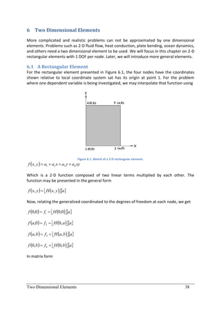
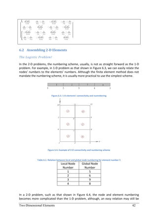
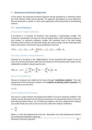
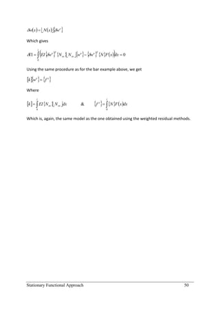
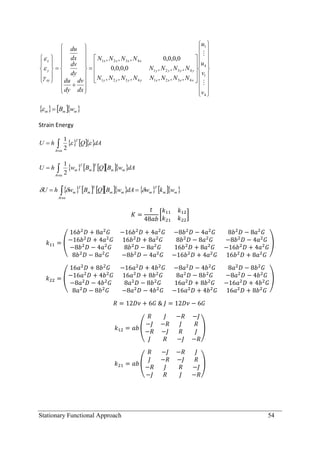
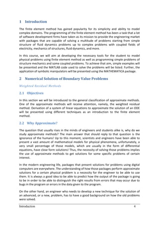
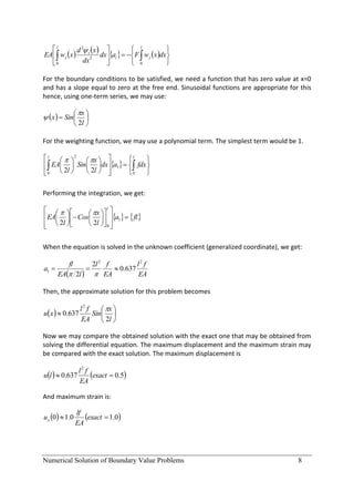
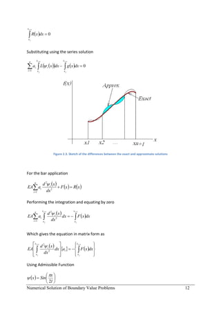
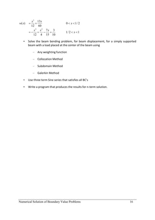
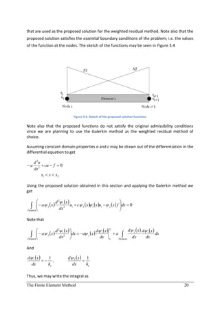
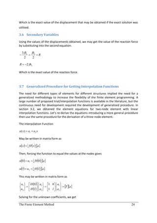
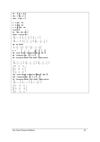
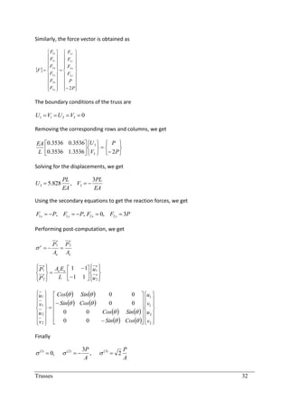
7.4 Finite Element Model of Plates in Bending

7.4.1 Displacement Function

The transverse displacement w(x,y), at any location x and y inside the plate element, is
expressed by

w( x, y)  H w a (‎ -1)
7

where H w  is a 64 element row vector and {a} is the vector of unknown coefficients. For
the plate element under consideration, the bending degrees of freedom associated with
each node are

 w 
 w   H   a 
 x   w   1 
 w   H w,x   a2 
   
(‎ -2)
7
 y   H w, y    
  2 w   H w,x , y  a16 
    
 xy 

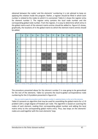
where Hw,i is the partial derivative of Hw with respect to i. Substituting the nodal coordinates
into equation (13), the nodal bending displacement vector {wb} is obtained as follows,

 wb    Tb  a  (‎ -3)
7

 w1 
 w1 
   H w 0,0  
 x   H 0,0 
 w1   w,x 
   H w, y 0,0  
where wb    y  [Tb ]    (‎ -4)
7
 H w,x , y 0,0 
2 &
w1
 
 xy    
    
  2 w4   H w,x , y 0, b 
 
 
 xy 

From equation (14), we can obtain

a  Tb 1wb  (‎ -5)
7

Substituting equation (16) into equation (12) gives


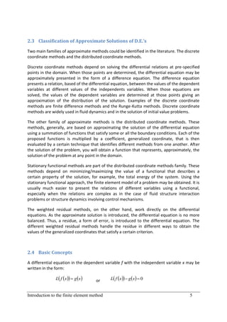
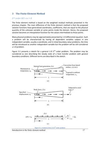
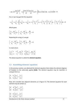
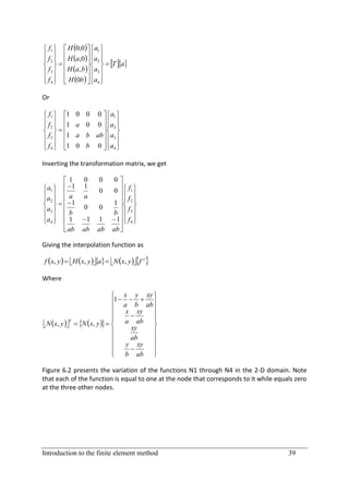
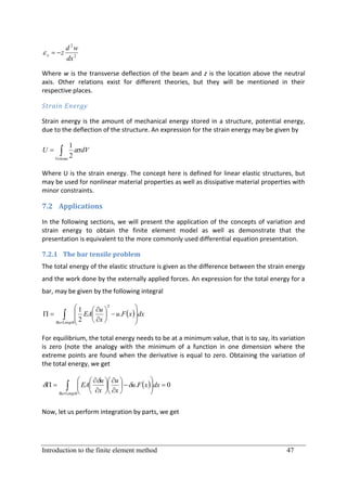
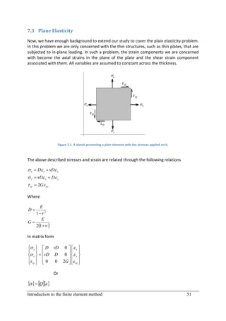
w( x, y)   H w  Tb   wb    N w  wb 
1
(‎ -6)
7

where [Nw] is the shape function for bending given by

 N w    H w  Tb 1 (‎ -7)
7

7.4.2 Strain-Displacement Relation

Consider the classical plate theory, for the strain vector {} can be written in terms of the
lateral deflections as follows

x 
     y   z 
  (‎ -8)
7
 
 xy 

where z is the vertical distance from the neutral plane and {} is the curvature vector which
can be written as,

 2w 
  2 
 2 x
  w 
     2    Cb  { a } (‎ -9)
7
 y2 
  w
 2 xy 
 

where

 Hw 
 , xx 
Cb     H w, yy  (‎ -10)
7
2 H 
 w, xy 

Substituting equation (17) into equation (23), gives

    Cb  Tb 1{wb }   Bb { wb } (‎ -11)
7

where

 Bb    Cb Tb 1 (‎ -12)
7

Thus, the strain-nodal displacement relationship can be written as


   z{ }  z Bb  wb  (‎ -13)
7

7.4.3 Constitutive Relations of Piezoelectric Lamina

The general form of the constitutive equation of the piezoelectric patch are written as
follows

 x   x 
   E  
 y  Q   e   y 
  T   (‎ -14)
7
 xy   e
    xy 

D
  E 
 

where,  x , y , xy are the stress in the x-direction, stress in the y-direction, and the planar
shear stress respectively;  x ,  y ,  xy are the corresponding mechanical strains; D is the
electric displacement (Culomb/m2), E is the electric field (Volt/m), e piezoelectric
material constant relating the stress to the electric field,  is the material dielectric
constant at constant stress (Farad/m), and Q  is the mechanical stress-strain constitutive
E

matrix at constant electric field. Q E is given by,

 E E 
1   2 12
0 
 E 
QE 
E
0 
1   12 
2

 E 
 0 0
21   
 

where E is the Young’s modulus of elasticity at constant electric field, and  is the Poisson’s
ratio.

Equation (28) can be rearranged as follows

 x   x 
   E
 y
  

Q   ee
T  
  e   y 
  (‎ -15)
7
 xy     e    xy 
T
 
E
  D
 


 x   x 
  D 
or   y   Q    y    eD (‎ -16)
7
   
 xy   xy 

 x 
 
E    e   y   D
T
and (‎ -17)
7
 
 xy 

1
where   .


7.4.4 Stiffness and Mass Matrices of the Element

The principal of virtual work states that

   U  T  W   0 (‎ -18)
7

where  is the total energy of the system, U is the strain energy, T is the kinetic energy, W
is the external work done, and (.) denotes the first variation.

7.4.4.1 The Potential Energy

The variation of the mechanical and electrical potential energies is given by

U      dV   D EdV
T
(‎ -19)
7
V V

where V is the volume of the structure. Substituting equation (30) and (31) into equation
(33) gives,

 
U  z T QD z    eD dV  D   eT z   D dV
    (‎ -20)
7
V V

Substituting from equations (20) and (27), we get,

U   z B w  Q z B  w    e N  w dV
T D
b b b b D D
V
(‎ -21)
7
   N w    e z B  w     N  w dV
T T
D D b b D D
V


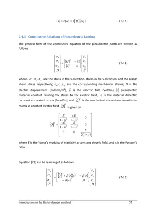
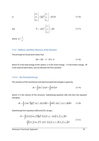
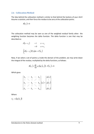
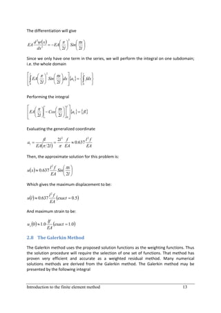
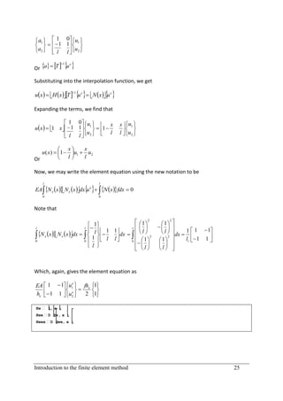
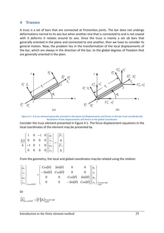
The terms of the expansion of equation (35) can be recast as follows

 z  B w  Q  B w dV  w   k w ,
2 T D T
b b b b b b b
V

  z B w   e N  wD dV  wb T  kbD  wD ,
T
b b D
V

    N
V
D wD T  eT z Bb  wb dV  wD T  k Db  wb   wD T  kbD T  wb  ,

and    N
V
D wD T  N D  wD dV  wD T  k D  wD ;

where [kb] is bending stiffness matrix, [kbD] is bending displacement-electric displacement
coupling matrix, and [kD] is the electric stiffness matrix.

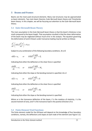
7.4.4.2 The Kinetic Energy

The variation of the kinetic energy T of the plate/piezo patch element is given by,

 2w 
A



T  w  h 2  dA
t 

(‎ -22)
7

where  is the density/equivalent density and h is the thickness of the element. The above
equation can be rewritten in terms of nodal displacements as follows

 
 2w 
dA  h wb T N w T N w wb  dA  wb T mb wb 

A
w  h


2 
t  A
  (‎ -23)
7

where [mb] is the element bending mass matrix.

7.4.4.3 The external work

The variation of the external work done exerted by the shunt circuit is given by

W    DLqdA
 (‎ -24)
7
A


where A is the element area, L is the shunted inductance, and q is the charge flowing in the
circuit. But, as the charge is the integral of the electric displacement over the element area;
then equation (38) reduces to,

W    DdA LDdA
 (‎ -25)
7
A A

Substituting from equation (20), gives

W  wD T  N D T dA N D LwD dA
 (‎ -26)
7
A A

which can be recast in the following form,

W   wD T mD wD 
  (‎ -27)
7

where [mD] is the element electric mass matrix.

Finally, the element equation of motion with no external forces can be written as

mb  0   wb   k b 
 k bD   wb  0
 0  w   k 
mD   D   Db

k D  wD  0
(‎ -28)
7
     


Introduction to the Finite Element Method

More Related Content

What's hot

Similar to Introduction to the Finite Element Method

More from Mohammad Tawfik

Introduction to the Finite Element Method