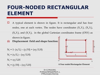
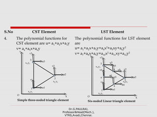
![DERIVATION OF STIFFNESS MATRIX
FOR 2-D ELEMENT (CST ELEMENT)
We know that stiffness matrix [K] for any element,
Stiffness matrix, [K] = [B]T
[D] [B] dv
v
= [B]T
[D] [B] v [ dv = v]
v
= [B]T
[D] [B] A x t [ v = A x t]
Stiffness matrix, [K] = [B]T
[D] [B] A x t
[t = Thickness of elements]
Dr.G.PAULRAJ,
Professor&Head(Mech.),
VTRS,Avadi,Chennai.](https://image.slidesharecdn.com/feaunit3-190403041846/85/Finite-Element-Analysis-UNIT-3-10-320.jpg)
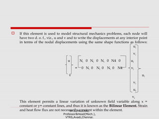
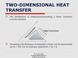
![1 x1 y1
Area of element A = (1/2) 1 x2 y2
1 x3 y3
β1 0 β2 0 β3 0
Strain displacement matrix, [B] = (1/2A) 0 γ1 0 γ2 0 γ3
γ1 β1 γ2 β2 γ3 β3
Where β1 = y2 –y3
β2 = y3 –y1
β3 = y1 –y2
γ1 = x3 – x2
γ2 = x1 – x3
γ3 = x2– x1
Dr.G.PAULRAJ,
Professor&Head(Mech.),
VTRS,Avadi,Chennai.](https://image.slidesharecdn.com/feaunit3-190403041846/85/Finite-Element-Analysis-UNIT-3-11-320.jpg)
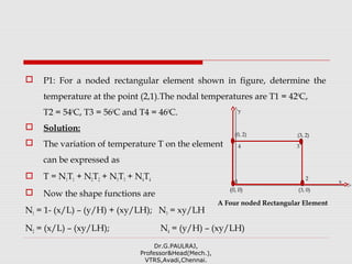
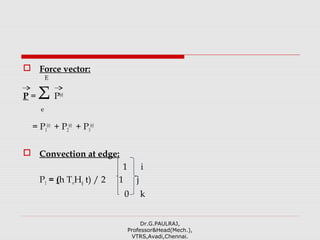
![ For plane stress problem,
1 v 0
[D] = E/(1-v2
) v 1 0
0 0 (1-v)/2
For plane strain problem,
1-v v 0
[D] = E/(1+v)(1-2v) v 1-v 0
0 0 (1-2v)/2
Dr.G.PAULRAJ,
Professor&Head(Mech.),
VTRS,Avadi,Chennai.](https://image.slidesharecdn.com/feaunit3-190403041846/85/Finite-Element-Analysis-UNIT-3-12-320.jpg)
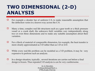
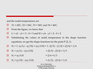
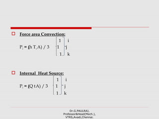
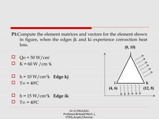
![ P1: For a triangular element shown in figure. Obtain the strain-
displacement relation matrix [B] and determine the strains ex, ey andγxy.
Nodal displacements are:
u1 = 0.001; v2 = -0.004
u2 = 0.003; v2 = 0.002
u3 = -0.002; v3 = 0.005
All co-ordinates are mm.
Solution:
x1 = 1mm ; y1 = 1mm
x2 = 8mm; y2 = 4mm
x3 = 2mm; y3 = 7mm
Dr.G.PAULRAJ,
Professor&Head(Mech.),
VTRS,Avadi,Chennai.
1
(1,1)
3
(2,7)
2
(8,4)
X
Y
O](https://image.slidesharecdn.com/feaunit3-190403041846/85/Finite-Element-Analysis-UNIT-3-13-320.jpg)
![ To find the element strain,
Normal strain, ex
Normal strain, ey
Shear strain, γxy
1 x1 y1 1 1 1
Area of element A = (1/2) 1 x2 y2 = (1/2) 1 8 4
1 x3 y3 1 2 7
= (1/2) [1x (56-8) – 1(7-4) + 1 (2-8)]
A = 19.5 mm
We know that, β1 0 β2 0 β3 0
Strain displacement matrix, [B] = (1/2A) 0 γ1 0 γ2 0 γ3 ----- (1)
γ1 β1 γ2 β2 γ3 β3
Dr.G.PAULRAJ,
Professor&Head(Mech.),
VTRS,Avadi,Chennai.](https://image.slidesharecdn.com/feaunit3-190403041846/85/Finite-Element-Analysis-UNIT-3-14-320.jpg)
![ β1 = y2 –y3 = 4-7 =-3
β2 = y3 –y1 = 7-1 = 6
β3 = y1 –y2 = 1-4 =-3
γ1 = x3 – x2 = 2-8 = -6
γ2 = x1 – x3 = 1-2 = -1
γ3 = x2– x1 = 8-1 = -7
Substituting the above values in equ 1.
-3 0 6 0 -3 0
[B] = (1/2x 19.5) 0 -6 0 -1 0 7
-6 -3 -1 6 7 -3
Dr.G.PAULRAJ,
Professor&Head(Mech.),
VTRS,Avadi,Chennai.](https://image.slidesharecdn.com/feaunit3-190403041846/85/Finite-Element-Analysis-UNIT-3-15-320.jpg)
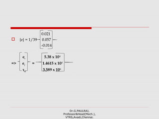
![ We know that,
u1
v1
Elemental strain, {e} = [B] {u} = [B] u2
v2
u3
v3
0.001
-0.004
-3 0 6 0 -3 0 0.003
{e} = (1/39) 0 -6 0 -1 0 7 0.002
-6 -3 -1 6 7 -3 -0.002
0.005
Dr.G.PAULRAJ,
Professor&Head(Mech.),
VTRS,Avadi,Chennai.](https://image.slidesharecdn.com/feaunit3-190403041846/85/Finite-Element-Analysis-UNIT-3-16-320.jpg)
![ Elemental stiffness matrix [k],
[ke
] = [k1
e
] + [k2
e
] + [k3
e
]
Conduction Edge convection Face convection
Conduction:
bi
2
+ ci
2
bibj+ cicj bibk+ cick
[k1] = kt/4A bjbi+ cjci bj
2
+ cj
2
bjbk+ cjck
bkbi+ ckci bkbj+ ckcj bk
2
+ ck
2
Dr.G.PAULRAJ,
Professor&Head(Mech.),
VTRS,Avadi,Chennai.](https://image.slidesharecdn.com/feaunit3-190403041846/85/Finite-Element-Analysis-UNIT-3-29-320.jpg)
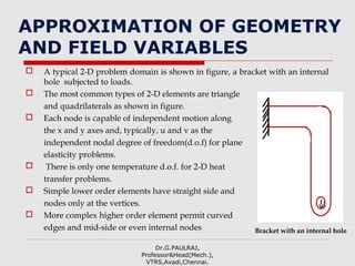
![ Edge Convection:
Edge ij :
2 1 0
[k2 ] = (h Hij t) / 6 1 2 0
0 0 0
Edge Length:
Hij = √ (x1 – x2)2
+ (y1– y2)2
Dr.G.PAULRAJ,
Professor&Head(Mech.),
VTRS,Avadi,Chennai.
x2, y2
x1, y1
x3, y3
i
k
j
h](https://image.slidesharecdn.com/feaunit3-190403041846/85/Finite-Element-Analysis-UNIT-3-30-320.jpg)
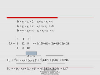
![Edge jk :
0 0 0
[k2 ] = (h Hjk t) / 6 0 2 1
0 1 2
Edge Length:
Hjk = √ (x2 – x3)2
+ (y2– y3)2
Where,
bi = yj – yk ci= xk – xj
bj = yk – yi cj= xi– xk
bk = yi – yj ck = xj – xiDr.G.PAULRAJ,
Professor&Head(Mech.),
VTRS,Avadi,Chennai.](https://image.slidesharecdn.com/feaunit3-190403041846/85/Finite-Element-Analysis-UNIT-3-31-320.jpg)
![1 x1 y1
Area of triangle 2A = 1 x2 y2
1 x3 y3
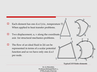
Face Convection:
2 1 1
[k3 ] = (h A) / 12 1 2 1
1 1 2
Dr.G.PAULRAJ,
Professor&Head(Mech.),
VTRS,Avadi,Chennai.
i
k
j
FaceConvection](https://image.slidesharecdn.com/feaunit3-190403041846/85/Finite-Element-Analysis-UNIT-3-32-320.jpg)
![ General FE representation is
bi
2
+ ci
2
bibj+ cicj bibk+ cick 2 1 0
[k1]=kt/4A bjbi+ cjci bj
2
+ cj
2
bjbk+ cjck +(h Hij t)/6 1 2 0
bkbi+ ckci bkbj+ ckcj bk
2
+ ck
2
0 0 0
2 1 1 1 i 1
+(h Hij t)/6 1 2 1 = (h T∞Hij t) / 2 1 j + (h T∞A) / 3 1
1 1 2 0 k 1
1
+ (Q t A)/3 1
[Assume t=1 unit in problems] 1Dr.G.PAULRAJ,
Professor&Head(Mech.),
VTRS,Avadi,Chennai.](https://image.slidesharecdn.com/feaunit3-190403041846/85/Finite-Element-Analysis-UNIT-3-35-320.jpg)
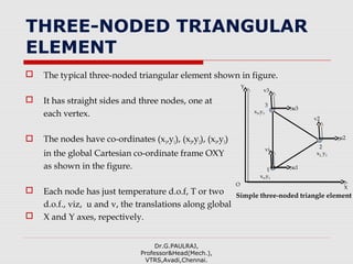
![ General FE equation for elemental evaluation:
Conduction:
bi
2
+ ci
2
bibj+ cicj bibk+ cick 25 -35 10
[k1] = kt/4A bjbi+ cjci bj
2
+ cj
2
bjbk+ cjck = -35 85 -50
bkbi+ ckci bkbj+ ckcj bk
2
+ ck
2
10 -50 40
Edge Convection:
2 0 1 0 0 0
[k1] = (hikHik)/6 0 0 0 + (hkjHkj)/6 0 2 1
1 0 2 0 1 2
Dr.G.PAULRAJ,
Professor&Head(Mech.),
VTRS,Avadi,Chennai.](https://image.slidesharecdn.com/feaunit3-190403041846/85/Finite-Element-Analysis-UNIT-3-38-320.jpg)
![2 0 1 0 0 0
[k2]=(15x8.25)/6 0 0 0 + (10x4.47)/6 0 2 1
1 0 2 0 1 2
41.25 0 20.625
[k2] = 0 14.9 7.45
20.625 7.45 56.15
Face Convection:
[k2] = 0 (No face convection)
Dr.G.PAULRAJ,
Professor&Head(Mech.),
VTRS,Avadi,Chennai.](https://image.slidesharecdn.com/feaunit3-190403041846/85/Finite-Element-Analysis-UNIT-3-39-320.jpg)
![ Force vector calculation:
P = P1
(e)
+ P2
(e)
+ P3
(e)
Convection at edges:
1 i 0
[P1] = (hikT∞Hik) /2 0 j + (hkjT∞Hkj) /2 1
1 k 1
2475
[P1] = 894
3369
Dr.G.PAULRAJ,
Professor&Head(Mech.),
VTRS,Avadi,Chennai.](https://image.slidesharecdn.com/feaunit3-190403041846/85/Finite-Element-Analysis-UNIT-3-40-320.jpg)
![ [P2] = 0 (No face convection)
1
[P3] = (Q tA) / 3 1
1
200
[P3] = 200
200
2675
P = P1
(e)
+ P2
(e)
+ P3
(e)
= 1094
3569
Dr.G.PAULRAJ,
Professor&Head(Mech.),
VTRS,Avadi,Chennai.](https://image.slidesharecdn.com/feaunit3-190403041846/85/Finite-Element-Analysis-UNIT-3-41-320.jpg)
![ The general FE representation is given as,
66.25 -35 30.625 T1 2675
[k] {T} = {P}=> -35 99.9 -42.55 T2 = 1094
30.625 -42.55 96.15 T3 3569
Dr.G.PAULRAJ,
Professor&Head(Mech.),
VTRS,Avadi,Chennai.](https://image.slidesharecdn.com/feaunit3-190403041846/85/Finite-Element-Analysis-UNIT-3-42-320.jpg)

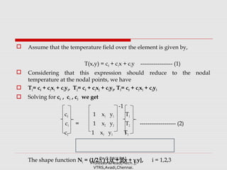
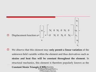
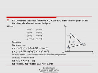
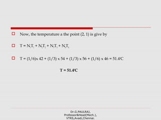
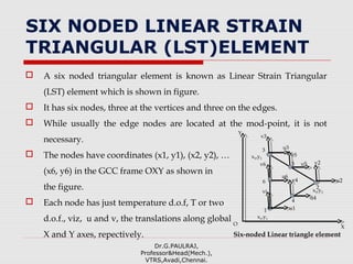
The document discusses two-dimensional finite element analysis. It describes triangular and quadrilateral elements used for 2D problems. The derivation of the stiffness matrix is shown for a three-noded triangular element. Shape functions are presented for triangular and quadrilateral elements. Examples are provided to calculate strains for a triangular element and to determine temperatures at interior points using shape functions.