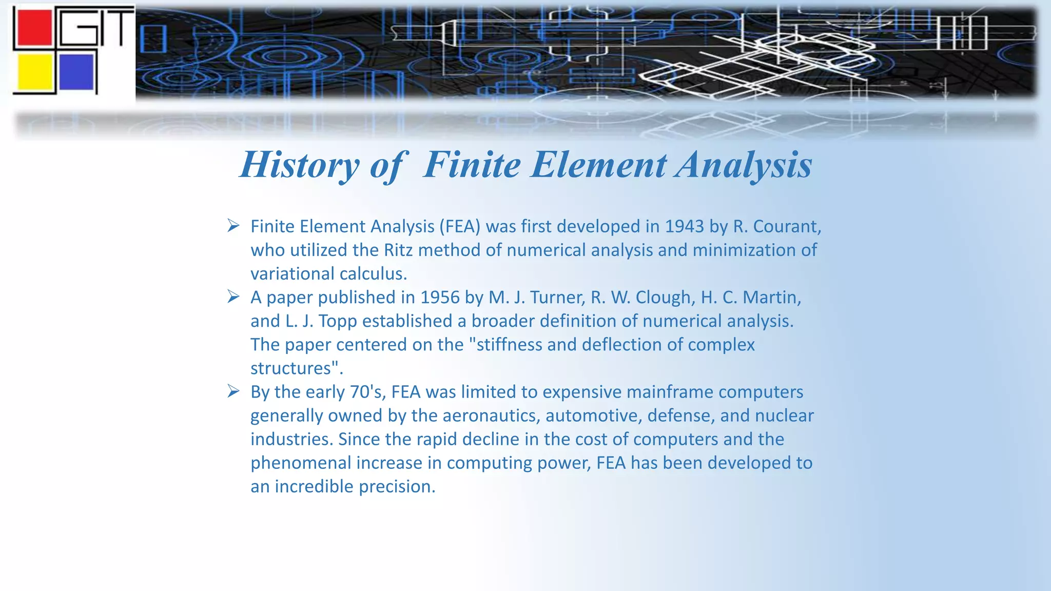
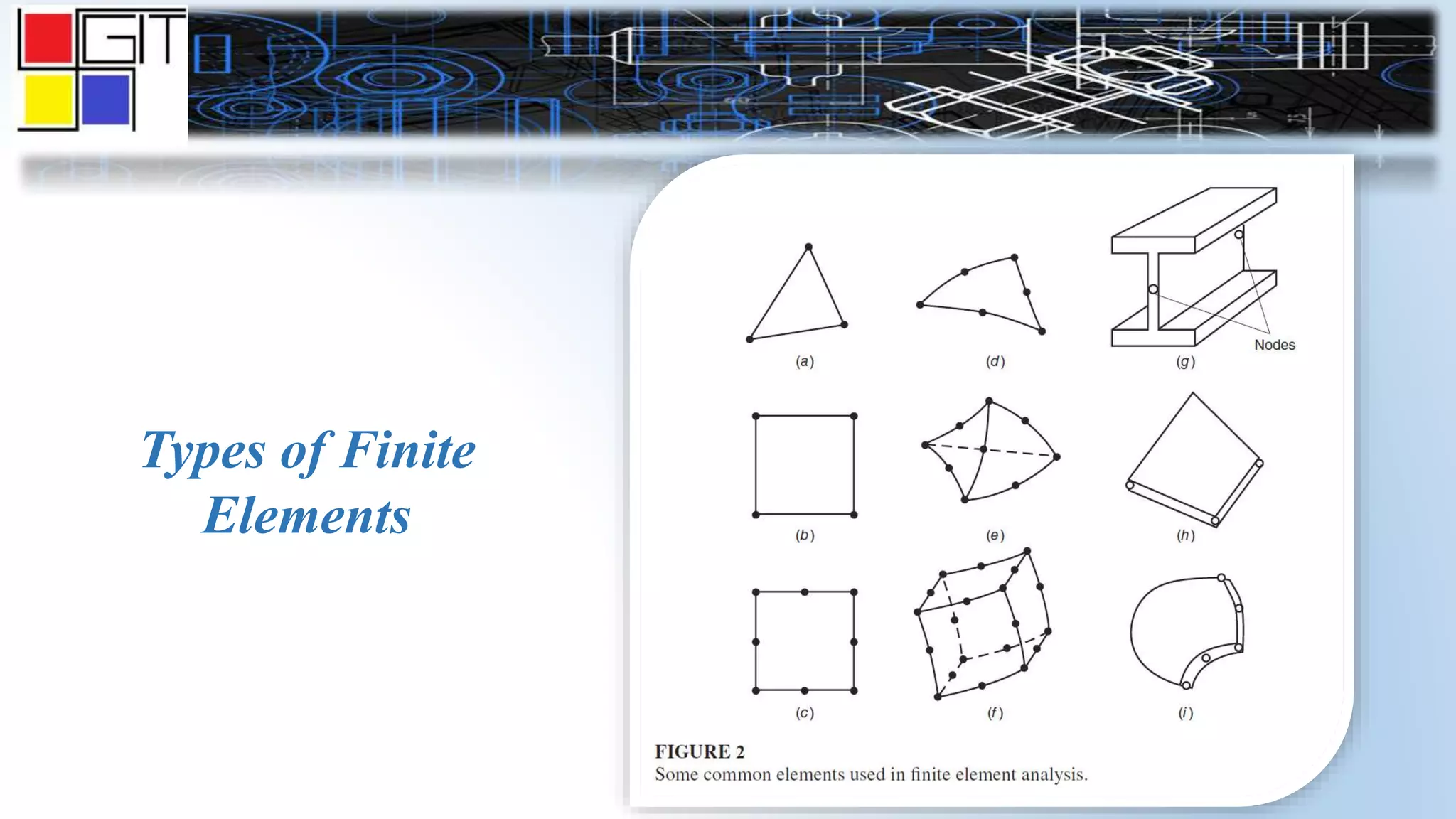
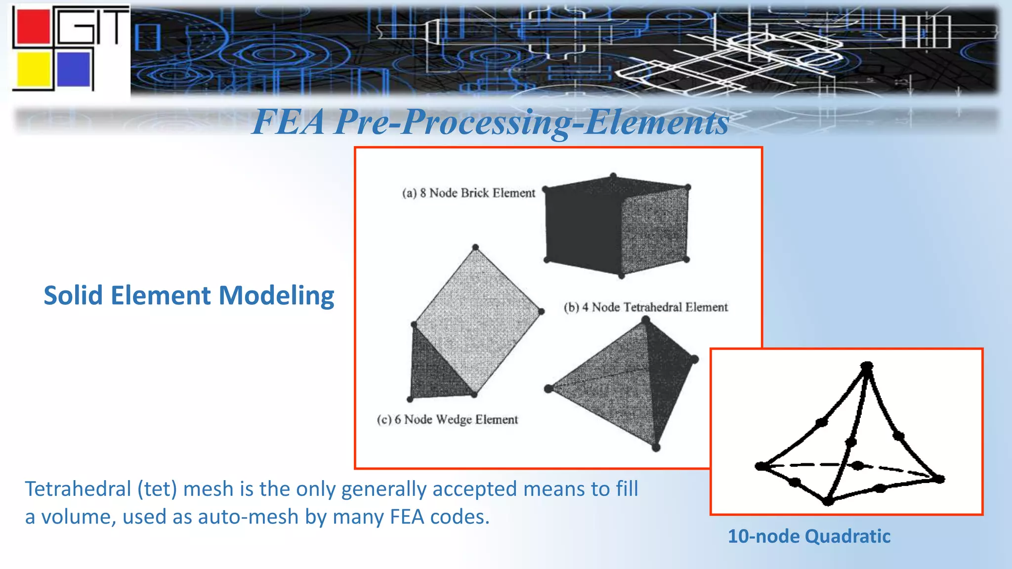
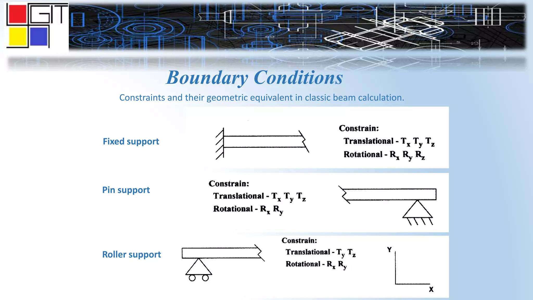
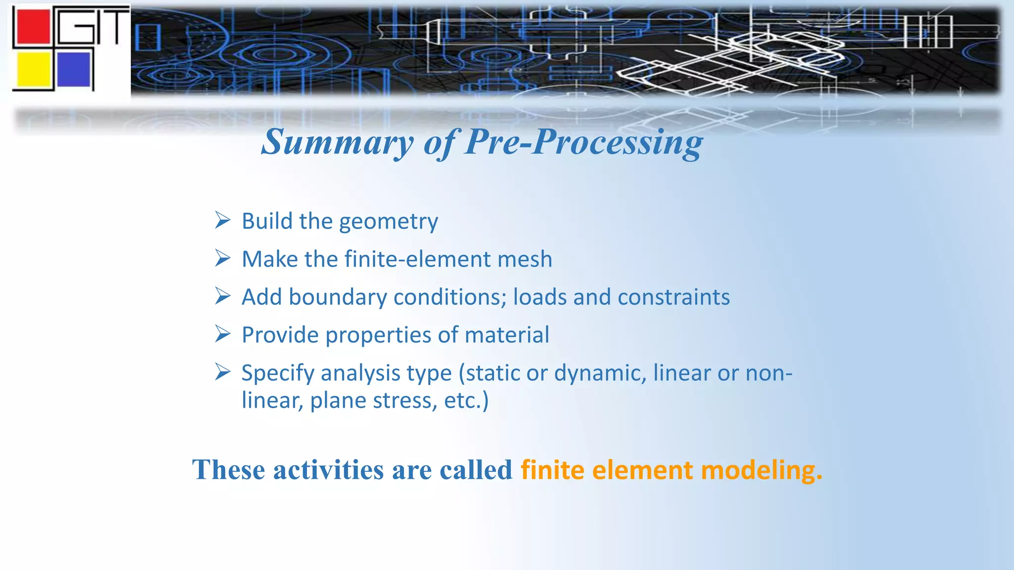
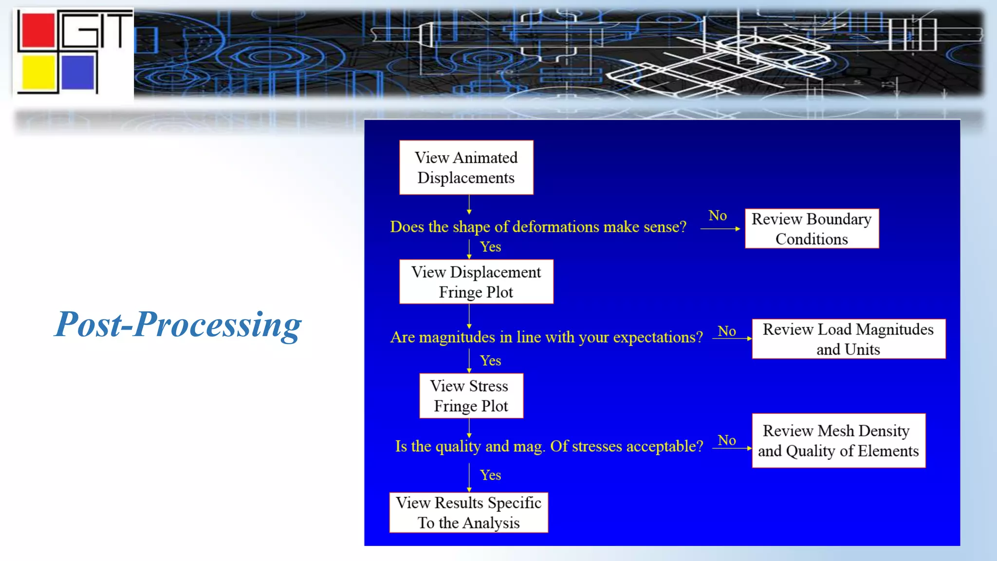
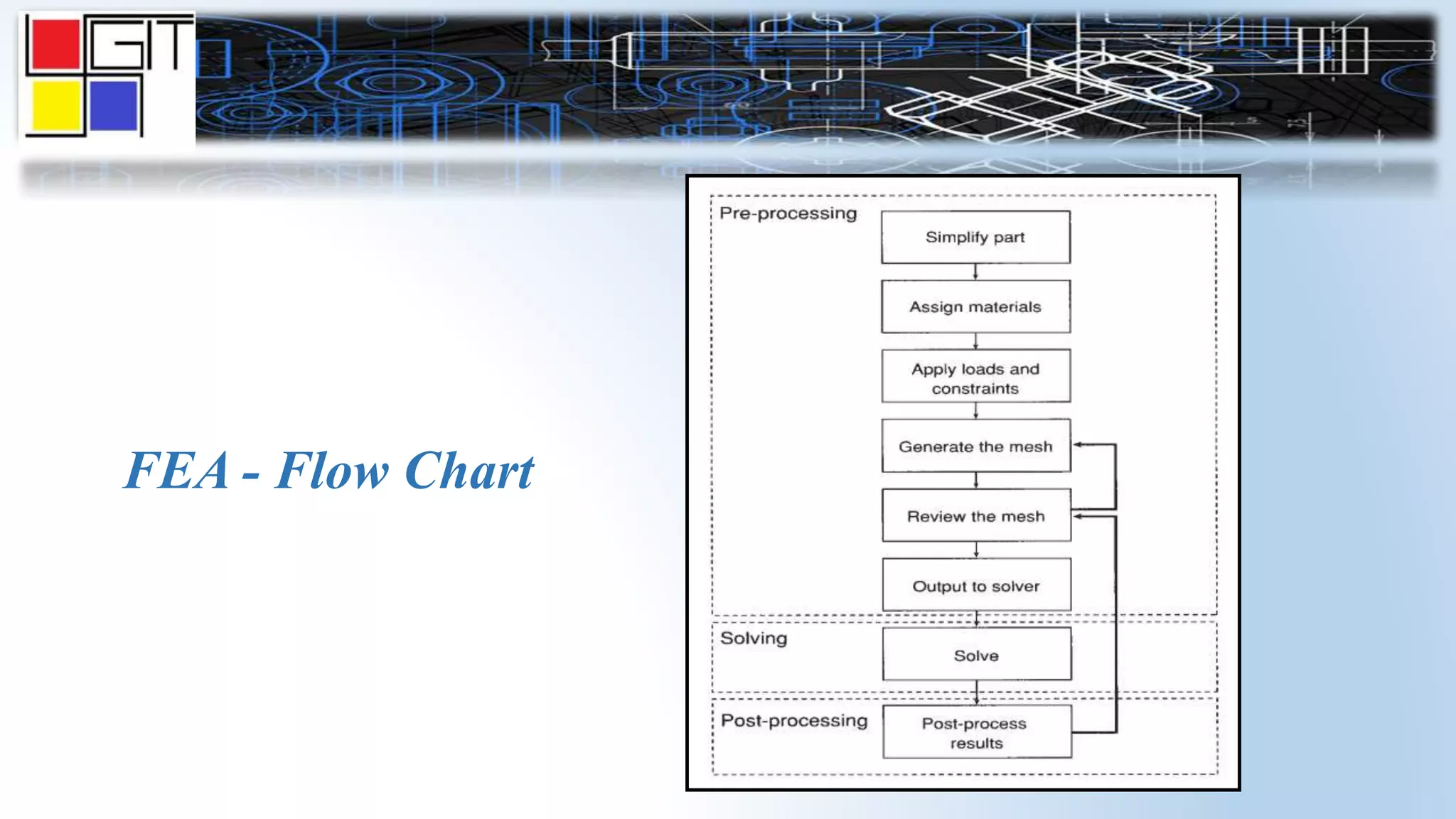
The document provides an overview of the history and basics of finite element analysis (FEA). It discusses how FEA was first developed in 1943 and expanded in the following decades. The basics section describes common FEA applications, basic steps which include converting differential equations to algebraic equations, element types, boundary conditions including loads and constraints, and pre-processing, solving, and post-processing steps. Key element types are also summarized.

1. GANDHINAGAR
INSTITUTE OF
TECHNOLOGY
Topic:- Finite Element Analysis
Guided by:-
Prof. Hardik Patel
Prepared by:-
Sonal S Upadhyay
110120119102

2. History of Finite Element Analysis
 Finite Element Analysis (FEA) was first developed in 1943 by R. Courant,
who utilized the Ritz method of numerical analysis and minimization of
variational calculus.
 A paper published in 1956 by M. J. Turner, R. W. Clough, H. C. Martin,
and L. J. Topp established a broader definition of numerical analysis.
The paper centered on the "stiffness and deflection of complex
structures".
 By the early 70's, FEA was limited to expensive mainframe computers
generally owned by the aeronautics, automotive, defense, and nuclear
industries. Since the rapid decline in the cost of computers and the
phenomenal increase in computing power, FEA has been developed to
an incredible precision.

3. Basics of Finite Element Analysis
FEA Applications
Evaluate the stress or temperature distribution in a mechanical
component.
Perform deflection analysis.
Analyze the kinematics or dynamic response.
Perform vibration analysis

4. Basic Steps
 First step: governing differential equation of the problem is converted into an integral form. These are two
techniques to achieve this :
(i) Variational Technique and
(ii) Weighted Residual Technique.
 Second step: the domain of the problem is divided into a number of parts, called as elements. Division of
the domain into elements is called a mesh.
 Third step: over a typical element, a suitable approximation is chosen for the primary variable of the
problem using interpolation functions (also called as shape functions) and the unknown values of the
primary variable at some pre-selected points of the element, called as the nodes.
Additional nodes are placed either on the boundaries or in the interior. The values of the primary variable
at the nodes are called as the degrees of freedom.

5. Basic Steps
 Fourth step: The approximation for the primary variable is substituted into the integral form. If the integral
form is of variational type, it is minimized to get the algebraic equations for the unknown nodal values of
the primary variable. If the integral form is of the weighted residual type, it is set to zero to obtain the
algebraic equations. In each case, the algebraic equations are obtained element wise first (called as the
element equations) and then they are assembled over all the elements to obtain the algebraic equations
for the whole domain (called as the global equations).
 Last step: The post-processing of the solution is done. That is, first the secondary variables of the problem
are calculated from the solution. Then, the nodal values of the primary and secondary variables are used
to construct their graphical variation over the domain either in the form of graphs (for 1-D problems) or 2-
D/3-D contours as the case may be.

6. Types of Finite
Elements

7. FEA Pre-Processing
 Mesh is your way of communicating geometry
to the solver, the accuracy of the solution is
primarily dependent on the quality of the
mesh.
 The better the mesh looks, the more accurate
the solution is.
 A good-looking mesh should have well-
shaped elements, and the transition between
densities should be smooth and gradual
without skinny, distorted elements.
Mesh

8. FEA Pre-Processing
Finite elements supported by most finite-element codes:

9. FEA Pre-Processing-Elements
Beam Elements
Beam elements typically fall into two
categories; able to transmit moments or not
able to transmit moments.
Rod (bar or truss) elements cannot carry moments.
The most general line element is a beam. (a) and (b) are higher order line elements.

10. FEA Pre-Processing-Elements
Plate and Shell Modeling
Plate and shell are used interchangeably and refer to surface-like elements used to represent thin-walled structures.
A quadrilateral mesh is usually more accurate than a mesh of similar density
based on triangles. Triangles are acceptable in regions of gradual transitions.

11. FEA Pre-Processing-Elements
Solid Element Modeling
Tetrahedral (tet) mesh is the only generally accepted means to fill
a volume, used as auto-mesh by many FEA codes.
10-node Quadratic

12. Boundary Conditions
Loads
Loads are used to represent inputs to the system. They can be in the forms of forces, moments, pressures, temperature, or
accelerations.
Constraints
Constraints are used as reactions to the applied loads. Constraints can resist translational or rotational deformation induced
by applied loads.
Linear Static Analysis
Boundary conditions are assumed constant from application to final deformation of system and all loads are applied gradually
to their full magnitude.
Dynamic Analysis
The boundary conditions vary with time.

13. Boundary Conditions
Non-linear Analysis
The orientation and distribution of the boundary conditions vary as displacement of the structure is calculated.
Degrees of Freedom
 Spatial DOFs refer to the three translational and three rotational modes of displacement that are possible for any part
in 3D space. A constraint scheme must remove all six DOFs for the analysis to run.
 Elemental DOFs refer to the ability of each element to transmit or react to a load. The boundary condition cannot load
or constrain a DOF that is not supported by the element to which it is applied.
 A solid face should always have at least three points in contact with the rest of the structure. A solid element should
never be constrained by less than three points and only translational DOFs must be fixed.
Accuracy
The choice of boundary conditions has a direct impact on the overall accuracy of the model.
Over-constrained model – an overly stiff model due to poorly applied constraints.

14. Boundary Conditions
Constraints and their geometric equivalent in classic beam calculation.
Pin support
Fixed support
Roller support

15. Summary of Pre-Processing
 Build the geometry
 Make the finite-element mesh
 Add boundary conditions; loads and constraints
 Provide properties of material
 Specify analysis type (static or dynamic, linear or non-
linear, plane stress, etc.)
These activities are called finite element modeling.

16. Solving the Model - Solver
Once the mesh is complete, and the properties and boundary
conditions have been applied, it is time to solve the model. In most
cases, this will be the point where you can take a deep breath, push
a button and relax while the computer does the work for a change.
Multiple Load and Constraint Cases
In most cases submitting a run with multiple load cases will be faster
than running sequential, complete solutions for each load case.
Final Model Check

17. Post-Processing

18. FEA - Flow Chart

19. GANDHINAGAR
INSTITUTE OF
TECHNOLOGY
Advantages of the finite element method over other
numerical methods
 The method can be used for any irregular-shaped domain and all types of boundary conditions.
 Domains consisting of more than one material can be easily analyzed.
 Accuracy of the solution can be improved either by proper refinement of the mesh or by choosing
approximation of higher degree polynomials.
 The algebraic equations can be easily generated and solved on a computer. In fact, a general purpose code
can be developed for the analysis of a large class of problems.