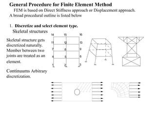
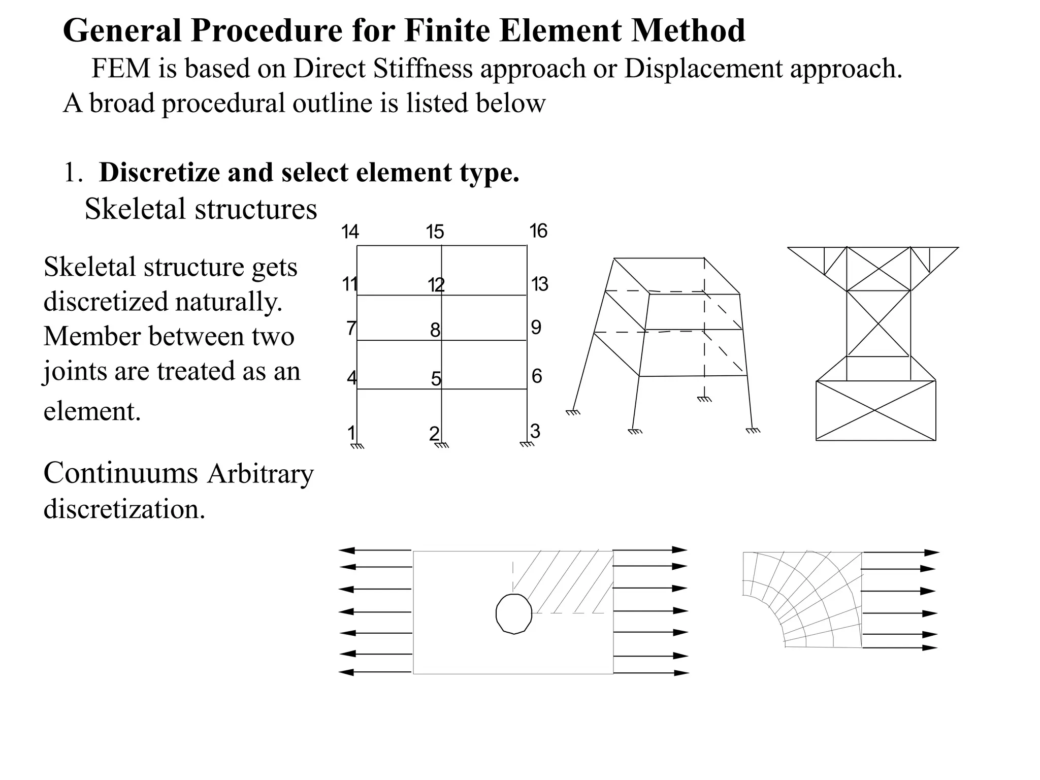
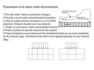
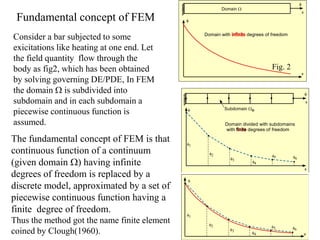
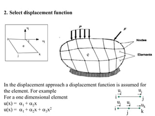
1. The general procedure for the finite element method involves discretizing the domain into elements, selecting displacement functions to approximate displacements within each element, and establishing relationships between displacements, strains, and stresses to set up the governing equations. 2. A displacement-based approach is used where shape functions are chosen to describe the displacement field within an element and ensure continuity of displacements between elements. 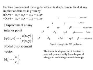3. The strain-displacement and stress-strain relationships are developed using the shape functions and material properties to create the elemental stiffness matrix which are then assembled in the global finite element model.

1. General Procedure for Finite Element Method
FEM is based on Direct Stiffness approach or Displacement approach.
A broad procedural outline is listed below
1. Discretize and select element type.
Skeletal structures
1 2 3
4 5 6
7 8 9
11 12 13
14 15 16
Skeletal structure gets
discretized naturally.
Member between two
joints are treated as an
element.
Continuums Arbitrary
discretization.

2. Precautions to be taken while discretization.
1.Provide nodes wherever geometry changes
2.Provide a set of nodes along bimaterial interface,
so that no single element encompass or cover both
materials. Element should cover one material.
3. Nodes at such points where concentrated load acts.
4.Nodes at points of specific interest for the analyst.
5.Nodes/|elements are provided such that distributed loads are covered completely
by the element edge. Distributed load shall not be applied partially on any element
edge.
Node where geometry
changes
Nodes along
bi-material interface
Material 1
Material 2

3. Precautions to be taken while discretization (contd)
6.Nodes to provide prescribed boundary condition.
7.Fine mesh in the regions of steep stress gradient.
8.Use symmetry condition
9 Aspect ratio of element1
10. Avoid obtuse/acute angle
11.Node numbering along shorter direction.
W
B
W /B>>1
W
B
W /B"1

4. f
x
f1
f2
f3 f4
f5 f6
x
f Subdomain We
Domain divided with subdomains
with degrees of freedom
Domain W
x
x
Domain with degrees of freedom
f
f
Fundamental concept of FEM
The fundamental concept of FEM is that
continuous function of a continuum
(given domain W) having infinite
degrees of freedom is replaced by a
discrete model, approximated by a set of
piecewise continuous function having a
finite degree of freedom.
Thus the method got the name finite element
coined by Clough(1960).
f6
f5
f4
f3
f2
f1
f
x
Consider a bar subjected to some
exicitations like heating at one end. Let
the field quantity flow through the
body as fig2, which has been obtained
by solving governing DE/PDE, In FEM
the domain W is subdivided into
subdomain and in each subdomain a
piecewise continuous function is
assumed.
Fig. 2

5. 2. Select displacement function
e
i
j k
l
e
ul
vl
In the displacement approach a displacement function is assumed for
the element. For example
For a one dimensional element
u(x) = a1 + a2x
u(x) = a1 + a2x + a3x2
i
ui uj
j
i
ui
k
uj
j
uk

6. For two dimensional rectangular elements displacement field at any
interior of element is given by
u(x,y) = a1 + a2x + a3y + a4xy
v(x,y) = a5 + a6x + a7y + a8xy
 
  i
i
i
Displacement at any
interior point
u(x,y)
(x,y)
v(x,y)
Nodal displacement
vector
u
d
v
 
   
 
 
  
 
1
x y
x2 xy y2
x2y xy2 y3
x3y x2y2 xy3 y4
x3
x4
Constant
Linear
Quadratic
Cubic
Quartic
Pascal triangle for 2D problems
The terms for displacement function is
selected symmetrically from the pascal
triangle to maintain geometric isotropy

7. x y
z
x2
y2
x3
x4
y3
y4
z2
z3
z4
xz
xy
x2z
xz2
x2y xy2
z2y
zy2
xyz
x3z
x2z2
xz3
y3z
y2z2
yz3
x3y x2y2 xy3
x2yz y2xz
z2yx
zy
Pascal triangle for 3D problems
 
i
i
j
i
j j
e
k k
l k
l
l
Element displacement vector
u
v
u
d
d v
d
d u
d v
u
v
 
 
 
 
 
 
 
   
 
   
   
   
 
 
 
 
 

8.  
1
2
3
4
( , ) 1
u x y x y xy
a
a
a
a
 
 
 
  
 
 
 
 
5
6
7
8
( , ) 1
v x y x y xy
a
a
a
a
 
 
 
  
 
 
 
 
   
1
2
3
4
5
6
7
8
u(x,y) 1 x y xy 0 0 0 0
(x,y)
v(x,y) 0 0 0 0 1 x y xy
1 x y xy 0 0 0 0
(x,y)
0 0 0 0 1 x y xy
a
 
 
a
 
a
 
 
a
     
  
   
  a
     
 
a
 
a
 
 
a
 
 
  a
 
 
(1a)
(1b)

9. i i i i
j j j j
k k k k
l l l l
Using the nodal conditions like
x x ,y y u(x,y) u ,v(x,y) v
x x ,y y u(x,y) u ,v(x,y) v
x x ,y y u(x,y) u ,v(x,y) v
x x ,y y u(x,y) u ,v(x,y) v
    
    
    
    
This results in as many conditions as the number of
unknown constants.
(2)

10. 1 1
1 1 1 1
1 2
1 1 1 1
2 3
2 2 2 2
2 4
2 2 2 2
3 5
3 3 3 3
6
3 3 3 3 3
7
4 4 4 4
4
8
4 4 4 4
4
1 0 0 0 0
0 0 0 0 1
1 0 0 0 0
0 0 0 0 1
1 0 0 0 0
0 0 0 0 1
1 0 0 0 0
0 0 0 0 1
u x y x y
v x y x y
u x y x y
v x y x y
u x y x y
v x y x y
x y x y
u
x y x y
v
a
a
a
a
a
a
a
a
  
 
  
 
  
 
  
 
  
 
  
 

  
 
  
 
  
 
  
 
   
    
 
 










 
 

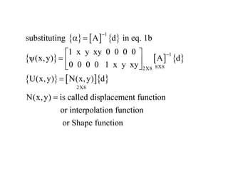
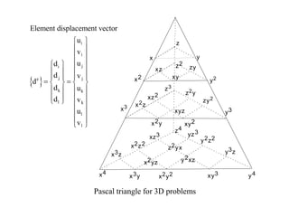
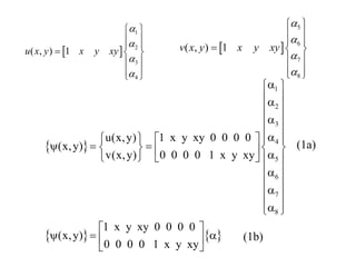
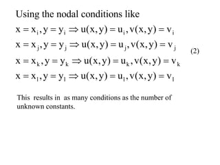
Using nodal boundary condition listed in eq. (2) in eq. 1a, following matrix
eqn. Can be obtained
    
     
1
(3)
d A
A d
a
a


     
For quadrilateral element [A] is of size 8 X 8

11.      
     
    
1
1
8X8
2X8
2X8
substituting A d in eq. 1b
1 x y xy 0 0 0 0
(x,y) A d
0 0 0 0 1 x y xy
U(x,y) N(x,y) d
N(x,y) is called displacement function
or interpolation function


a 
 
   
 


or Shape function

12.  
i
i
i j k l
j
i j k l
i
i
u
v
N , 0, N , 0, N , 0, N , 0
(x,y) u
0, N , 0, N , 0, N , 0, N
.
.
Properties of shape function
N 1.0 at node 'i', and zero at all other nodes
N 0 at all the
 
 
 
  
   
 
  
 
 
 


n
i
i 1
sides on which node of interest does not fall.
N 1.0, n = number of nodes per element

 

13.         
    
x
y
xy
3X2 2X8
3X8
u
, 0
x x
u
v
0,
v
y y
u v
,
y x y x
L (x, y) L N(x, y) d
B d
   
 
   
 
     

   
 
   
  
     
 
   
     

   
   
 

   
   
   
   
 
3. Establish strain displacement and stress/strain relationship.
 
( )
x
du d
u x
dx dx

 
   
 
For one dimensional element
For two dimensional element

14.  
       
   
 
 
0 0
0
N
, 0
x
N
B 0,
y
N N
,
y x
For a linear elastic behavior the relationship
between stresses and strains are of the form
D
D Elasticity matrix
initial strain ve
 

   
 

 

 
    
 

 
 
 
  
 
 
 
      

 
 
0
ctor (thermal strain T)
initial residual stresses
a
 

15.    
       
   
       
   
 
         
   
          
       
            
e
e
e e
e
e
e e
T
e
v
0 0
T
e
0 0
v
T T
e
0
v v
T
0
v
T T
e
v
T T
T T
0 0
v v
Internal virtual energy U = dv
substitute D in above eqn.
U = D dv
U = D dv D dv
dv
B d , = B d
U = d B D B d dv
- d B D dv d B dv
   
      
       
       
   
    
 
    


 


 
4. Establish equilibrium equation to develop element stiffness relation.
Virtual work principle of a deformable body in equilibrium is subjected to arbitrary
virtual displacement satisfying compatibility condition (admissible displacement), then
the virtual work done by external(loads will be equal to virtual strain energy of internal
stresses. e e
U W
 


16. px
py
x
y
Surface traction
i j
k
l
px
x
y
bx
by
Body force
i j
l
y
l
k
j
i
Pxl
Pxk
Pxj
Pyl
Pyk
Pyi
Nodal force
       
       
e e
T T T x
e
b
y
v v
T T T x
e
s
y
s s
External virtual workdue to body force
b
w = (x, y) b dv d N dv
b
External virtual work due to surface force
p
w = (x, y) p dv d N dv
p
External virtual work due to nodal f
 
      
 
 
      
 
 
 
       
T
T
e e e
c xi yi xj yj
orces
w d P , P = P , P , P , P ,....
  

17. For equilibrium internal virtual work = external virtual work
             
   
       
    
      
 
e e
e
e
e
T T T
0
v v
T
0
v
T T T
x x e
y y
s
v
e
e e
T
e
v
e
d ( B D B dv d - B D dv
B dv)
b p
d N dv N dv P
b p
K d f
where
K B D B dv Element stiffness matrix
f Total nodal force vector
 
  
 
   
  
 
   
 
   
 
 
 

 

 


18.       
          
     
e
e e
e
T
e
v
T T
e 0 0
v v
T T
x x e
y y
s
v
where
K B D B dv
f B D dv B dv)
b p
N dv N dv P
b p

   
   
 
   
   

 
 
First term in {fe} is equivalent nodal force vector due to initial
strain. Second term is equivalent nodal force vector due to
initial stress. Third term is equivalent nodal force vector due to
body force. Fourth term is equivalent nodal force vector due to
surface traction. Last term is applied concentrated load vector