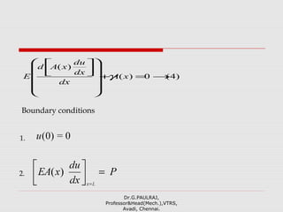
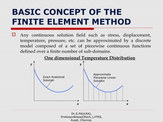
![WEIGHTED RESIDUAL…,
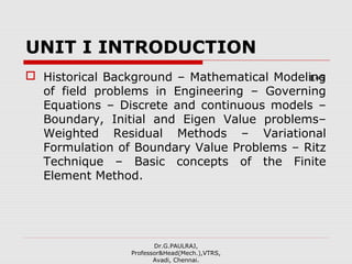
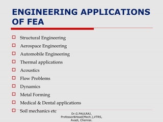
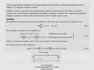
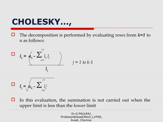
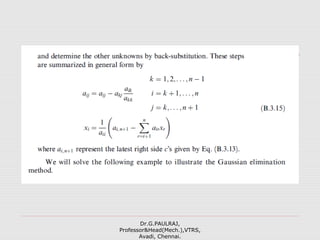
Galerkin’s method: Galerkin’s method uses the same functions
for Wi(x) that were used in the approximating equation. This
approach is the basis of the finite element method for problems
involving first-derivative terms. This methods yields the same
result as the variational method when applied to differential
equations that are self-adjoint.
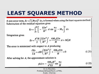
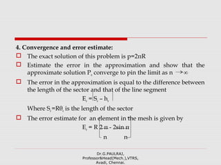
Least Squares method: The least squares method utilizes the
residual as the weighting function and obtains a new error term
defined by H
Er = [R(x)]2
d
0
This error is minimized w.r.t the unknown coefficient in the
approximate solution.
Dr.G.PAULRAJ,
Professor&Head(Mech.),VTRS,
Avadi, Chennai.](https://image.slidesharecdn.com/feaunit1-190403041842/85/Finite-Element-Analysis-UNIT-1-23-320.jpg)

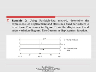
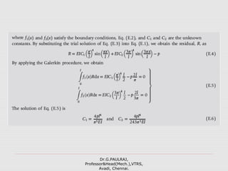
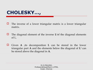
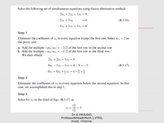

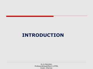
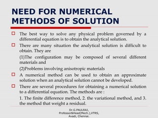
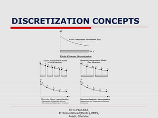
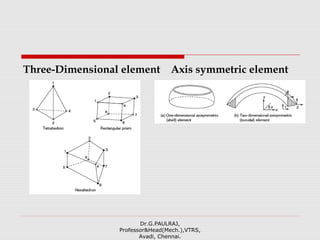
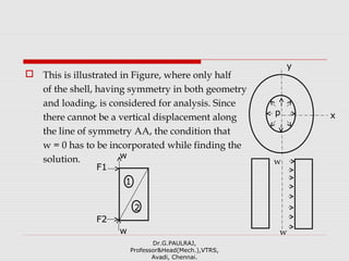
![ The approximating functions are defined in terms of field
variables of specified points called nodes or nodal points. Thus
in the finite element analysis the unknowns are the field
variables of the nodal points. Once these are found the field
variables at any point can be found by using interpolation
functions.
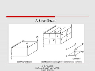
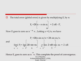
After selecting elements and nodal unknowns next step in finite
element analysis is to assemble element properties for each
element. For example, in solid mechanics, we have to find the
force-displacement i.e. stiffness characteristics of each individual
element. Mathematically this relationship is of the form
[k]e {δ}e= {F}e
where [k]e is element stiffness matrix, {δ }e is nodal displacement
vector of the element and {F}e is nodal force vector.Dr.G.PAULRAJ,
Professor&Head(Mech.),VTRS,
Avadi, Chennai.](https://image.slidesharecdn.com/feaunit1-190403041842/85/Finite-Element-Analysis-UNIT-1-78-320.jpg)
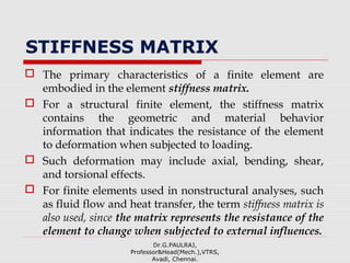
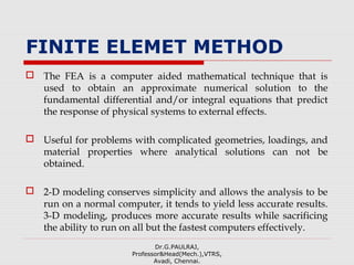
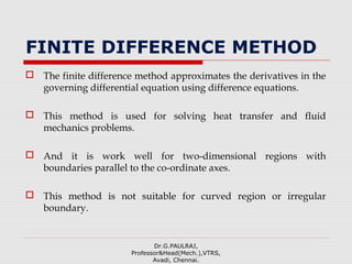
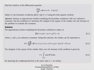
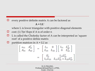
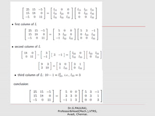
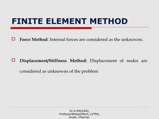
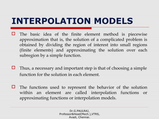
![MATRIX DISPLACEMENT
EQUATION
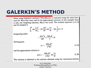
The standard form of matrix displacement equation is,
[k] {δ} = {F}
where [k] is stiffness matrix
{δ} is displacement vector and
{F} is force vector in the coordinate directions
The element kij of stiffness matrix maybe defined as the force at
coordinate i due to unit displacement in coordinate direction j.
Dr.G.PAULRAJ,
Professor&Head(Mech.),VTRS,
Avadi, Chennai.](https://image.slidesharecdn.com/feaunit1-190403041842/85/Finite-Element-Analysis-UNIT-1-82-320.jpg)
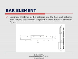
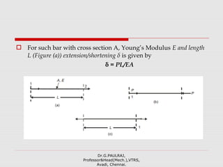
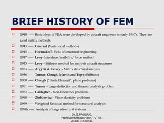
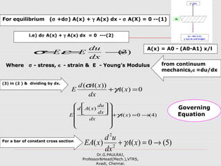
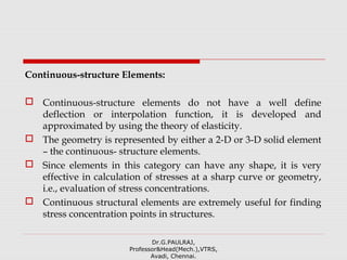
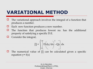
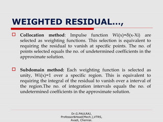
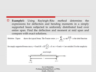
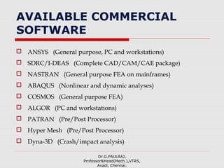
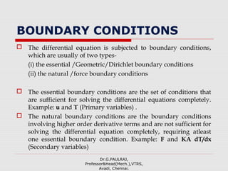
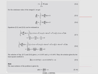
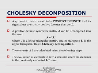
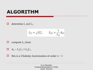
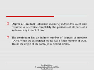
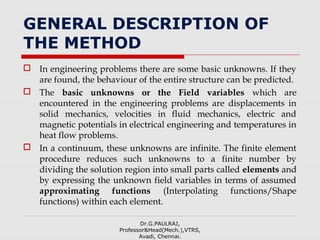
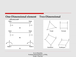
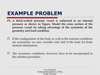
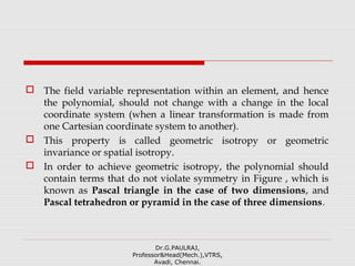
![ ∴ P=(EA/L)δ
∴ If δ = 1, P=EA/L
By giving unit displacement in coordinate direction 1, the forces
development in the coordinate direction 1 and 2 can be found
(Figure(b)). Hence from the definition of stiffness matrix,
k11 = E A/L and k21 = -E A/L
Similarly giving unit displacement in coordinate direction 2 (refer
Figure(c)), we get
k21 = -E A/L and k22 = E A/L
Thus, [k] = E/L 1 -1
-1 1
Dr.G.PAULRAJ,
Professor&Head(Mech.),VTRS,
Avadi, Chennai.](https://image.slidesharecdn.com/feaunit1-190403041842/85/Finite-Element-Analysis-UNIT-1-85-320.jpg)
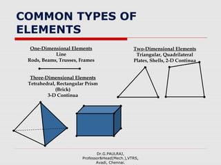
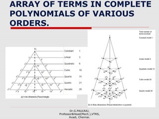

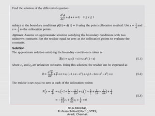
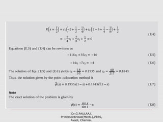
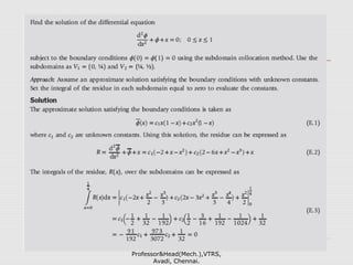
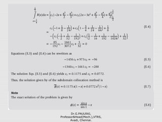
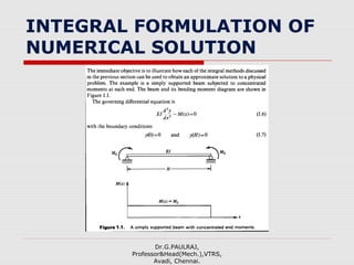
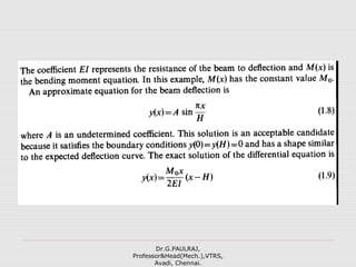
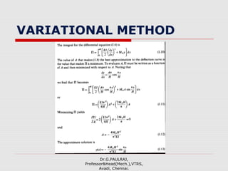
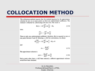
The document provides an introduction to the finite element method (FEM). It discusses that FEM is a numerical technique used to approximate solutions to boundary value problems defined by partial differential equations. It can handle complex geometries, loadings, and material properties that have no analytical solution. The document outlines the historical development of FEM and describes different numerical methods like the finite difference method, variational method, and weighted residual methods that FEM evolved from. It also discusses key concepts in FEM like discretization into elements, node points, and interpolation functions.