This document provides an overview of the finite element method (FEM) for a course on engineering geology. It outlines the course content, which includes an introduction to FEM, the Ritz-Galerkin and weak form methods, and applying FEM to 1D and 2D problems. Key aspects of FEM discussed include reducing partial differential equations to a system of algebraic equations, dividing problems into finite elements, and constructing approximate functions and element matrices. The origins and importance of FEM for solving complex problems are also summarized.

1. FEM
Collected by
Jyoti Anischit
MSc Engineering Geology.
III semester.

2. Course Content
• Introduction, Definition of Finite Element Method,
Differential Equation and Weak Form, Variational
Principal,
• Ritz‐Galerkin Method (approximate function, Galerkin
Method and Ritz Method), Finite Element Method (1‐D
• Problem): Construction of approximate function,
Element matrix, Total element matrix and simple
example,
• Finite Element Method (2‐D Problem): Construction of
approximate function, Element matrix & total element
• matrix, simple example and Gauss’s method of
elimination.

3. Finite Element Method – Introduction
• The Finite Element Method (FEM) is a numerical
method of solving systems of partial differential
equations (PDEs)
• It reduces a PDE system to a system of algebraic
equations that can be solved using traditional linear
algebra techniques.
• In simple terms, FEM is a method for dividing up a
very complicated problem into small elements that
can be solved in relation to each other.

4. “…The laws of nature are written in the language of
mathematics. These often take the form of ordinary or
partial differential equations.
The electronic digital computer is an amazingly fast
calculating tool; but it can handle only arithmetic.
– G. S. Ramaswamy
in “Design and Construction of
Concrete Shell Roofs”
Finite Element techniques do precisely this.”
The differential equation governing the physical
phenomena… have therefore to be reduced to a system of
simultaneous equation, before the computer can solve
then by a series of arithmetical operations.

5. 5
Where FEM started from…

6. 6
Where FEM started from…
1) The first paper in FEM:
• M. J. Turner, R. W. Clough, H. C. Martin & L. J. Topp,
“Stiffness and Deflection Analysis of Complex
Structures”, J. Aeronautical Science 23 (9), pp. 805-823,
Sept. 1956.
2) The coining of the name ‘Finite Element Method’:
• R. W. Clough, “The Finite Element Method in Plane Stress
Analysis”, Proc. 2nd ASCE Conf. On Electronic Computation,
Pittsburg, Sept. 1960.

7. 7
Where FEM started from…
3) Introduction of Isoparametric elements that made
FEM so very versatile:
• B. M. Irons & O. C. Zienkiewicz, “The Isoparametric Finite
Element System – A New Concept in Finite Element
Analysis”, Proc. Conf. Recent Advances in Stress Analysis,
Royal Aeronautical Society, London, 1968.
4) SAP-IV -- the first FEM Package :
• K. J. Bathe, E. L. Wilson & F. E. Peterson, “SAP IV – A
Structural Analysis Program for Static and Dynamic
Response of Linear Systems”, Report No. 73/11, Earthquake
Engineering Research Center, June 1973.

9. F.E.M.
• In finite element method, the structure to be
analyzed is subdivided into a mesh of finite-
sized elements of simple shape, and then the
whole structure is solved with quite easiness.
Rectangular Body Circular Plate
Finite Sized Element

10. Finite Sized Elements
• The rectangular panel in the rectangular body
and triangular panel in the circular plate are
referred to an ‘element’.
• There’re one-, two- and three-dimensional
elements.
• The accuracy of the solution depends upon
the number of the finite elements; the more
there’re, the greater the accuracy.

11. Finite Element of a Bar
• If a uniaxial bar is part of a structure then it’s
usually modeled by a spring element if and
only if the bar is allowed to move freely due to
the displacement of the whole structure. (One
dimensional element)
Bar
Spring element

12. Types of Elements
• Here goes the examples of two- and three-
dimensional finite sized elements.
Triangle
Rectangle
Hexahedron

13. Node
• The points of attachment of the element to
other parts of the structure are called nodes.
• The displacement at any node due to the
deformation of structure is known as the
nodal displacement.
Node

14. Why F.E.M.?
Simple trusses can be solved by just using the
equilibrium equations. But for the complex
shapes and frameworks like a circular plate,
equilibrium equations can no longer be applied as
the plate is an elastic continuum not the beams or
bars as the case of normal trusses.
Hence, metal plate is divided into finite
subdivisions (elements) and each element is
treated as the beam or bar. And now stress
distribution at any part can be determined
accurately.

15. Why F.E.M.?

18. Simple Bar Analysis
• Consider a simple bar made up of uniform
material with length L and the cross-sectional
area A. The young modulus of the material is
E.
• Since any bar is modeled as spring in FEM thus
we’ve:
L
F1 F2x1
x2k

19. Simple Bar Analysis
• Let us suppose that the value of spring constant is
k. Now, we’ll evaluate the value of k in terms of
the properties (length, area, etc.) of the bar:
We know that:
i.e.
Also: i.e.
And i.e.

20. Simple Bar Analysis
• Now substituting the values of x and F is the
base equation of k, we’ll have:
But
Hence, we may write:

21. Simple Bar Analysis
• According to the diagram, the force at node x1
can be written in the form:
• Where x1 – x2 is actually the nodal displacement
between two nodes. Further:
• Similarly:

22. Simple Bar Analysis
• Now further simplification gives:
• These two equations for F1 and F2 can also be
written as, in Matrix form:
• Or:

23. Simple Bar Analysis
• Here Ke is known as the Stiffness Matrix. So a
uniform material framework of bars, the value of
the stiffness matrix would remain the same for all
the elements of bars in the FEM structure.

24. Further Extension
• Similarly for two different materials bars joined
together, we may write:
;
F1 F2
x1 x2
k1
x3
F3
k2

25. Differential Equation
A Differential Equation is an equation containing the derivative of one or more
dependent variables with respect to one or more independent variables.
For example,

26. Classifiation by Type:
Ordinary Differential Equation
If a Differential Equations contains only ordinary derivatives of one or more
dependent variables with respect to a single independent variables, it is said to be an
Ordinary Differential Equation or (ODE) for short.
For Example,
Partial Differential Equation
If a Differential Equations contains partial derivatives of one or more dependent
variables of two or more independent variables, it is said to be a Partial Differential
Equation or (PDE) for short.
For Example,

27. Classifiation by Order:
The order of the differential equation (either ODE or PDE) is the order of the highest
derivative in the equation.
For Example,
Order = 3
Order = 2
Order = 1
General form of nth Order ODE is
= f(x,y,y1,y2,….,y(n))
where f is a real valued continuous function.
This is also referred to as Normal Form Of nth Order Derivative
So, when n=1, = f(x,y)
when n=2, = f(x,y,y1) and so on …

28. Importance
• FEM has become very familiar in subdivision of
continuum. It gives reliable and accurate results if
the number of elements are kept greater.
• Modern computer technology had helped this
analysis to be very easy and less time consuming.
• Large structures under loadings are now easily
solved and stresses on each and every part are
now being determined.

29. Galerkin method
• Galerkin suggested that the residue should be
multiplied by a weighting function that is a
part of the suggested solution then the
integration is performed over the whole
domain!!!
• Actually, it turned out to be a VERY GOOD idea

30. Galerkin Method
• Engineering problems: differential equations with
boundary conditions.
• Generally denoted as: D(U)=0; B(U)=0
• Our task: to find the function U which satisfies the
given differential equations and boundary conditions.
• Reality: difficult, even impossible to solve the problem
analytically
• In practical cases we often apply approximation.
• One of the approximation methods:
• Galerkin Method, invented by Russian mathematician
Boris Grigoryevich Galerkin.

31. 1D Rod Elements
• To understand and solve 2D and 3D problems we
must understand basic of 1D problems.
• Analysis of 1D rod elements can be done using
Rayleigh-Ritz and Galerkin’s method.
• To solve FEA problems same are modified in the
Potential-Energy approach and Galerkin’s
approach

32. 1D Rod Elements
• Loading consists of three types : body force f ,
traction force T, point load Pi
• Body force: distributed force , acting on every
elemental volume of body i.e. self weight of
body.
• Traction force: distributed force , acting on
surface of body i.e. frictional resistance,
viscous drag and surface shear

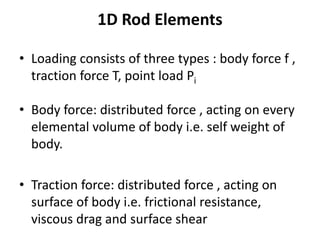
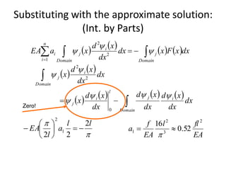
33. 1D Rod Elements
• Element strain energy
• Element stiffness matrix
• Load vectors
– Element body load vector
– Element traction-force vector
qkqU eT
e

][
2
1










11
11
][
e
eee
l
AE
k







1
1
2
flA
f eee








1
1
2
ee Tl
T

Element -1 Element-2

34. Bar application
   

n
i
ii xaxu
1

  02
2



xF
x
u
EA
     xRxF
dx
xd
aEA
n
i
i
i 1
2
2

Applying Galerkin method
         
 Domain
j
n
i Domain
i
ji dxxFxdx
dx
xd
xaEA 


1
2
2

35. In Matrix Form
         

















 Domain
ji
Domain
i
j dxxFxadx
dx
xd
xEA 

 2
2
Solve the above system for the “generalized
coordinates” ai to get the solution for u(x)

36. Same conditions on the functions are
applied
• They should be at least twice differentiable!
• They should satisfy all boundary conditions!
• Let’s use the same function as in the
collocation method:
  






l
x
Sinx
2



37. Substituting with the approximate solution:
         
 Domain
j
n
i Domain
i
ji dxxFxdx
dx
xd
xaEA 


1
2
2




























l
l
fdx
l
x
Sin
dx
l
x
Sin
l
x
Sina
l
EA
0
0
1
2
2
222



 ll
a
l
EA
2
22
1
2







EA
fll
EA
f
a
2
3
2
1 52.0
16



38. Substituting with the approximate solution:
(Int. by Parts)
         
 Domain
j
n
i Domain
i
ji dxxFxdx
dx
xd
xaEA 


1
2
2

 ll
a
l
EA
2
22
1
2







EA
fll
EA
f
a
2
3
2
1 52.0
16


   
       



Domain
ij
l
i
j
Domain
i
j
dx
dx
xd
dx
xd
dx
xd
x
dx
dx
xd
x




0
2
2
Zero!

39. What did we gain?
• The functions are required to be less
differentiable
• Not all boundary conditions need to be
satisfied
• The matrix became symmetric!

40. The Finite Element Method
2nd order DE’s in 1-D

41. Objectives
• Understand the basic steps of the finite
element analysis
• Apply the finite element method to second
order differential equations in 1-D

42. The Mathematical Model
• Solve:
• Subject to:
Lx
fcu
dx
du
a
dx
d








0
0
  00 ,0 Q
dx
du
auu
Lx









43. Step #1: Discretization
• At this step, we divide
the domain into
elements.
• The elements are
connected at nodes.
• All properties of the
domain are defined at
those nodes.

44. Step #2: Element Equations
• Let’s concentrate our
attention to a single
element.
• The same DE applies on
the element level, hence,
we may follow the
procedure for weighted
residual methods on the
element level!
21
0
xxx
fcu
dx
du
a
dx
d








   
21
2211
21
,
,,
Q
dx
du
aQ
dx
du
a
uxuuxu
xxxx















45. Conclusion
• Good at Hand Calculations, Powerful
when applied to computers
• Only limitations are the computer
limitations