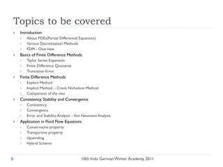
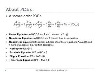
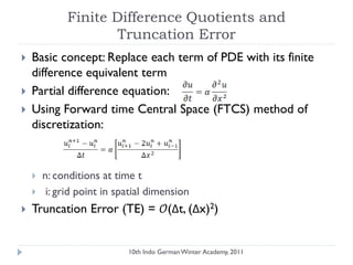
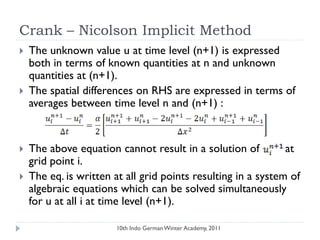
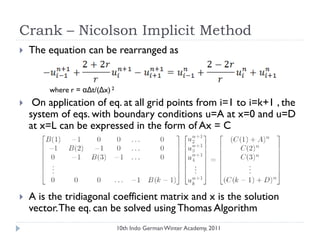
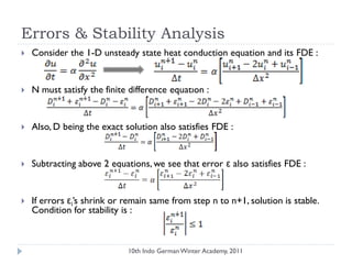
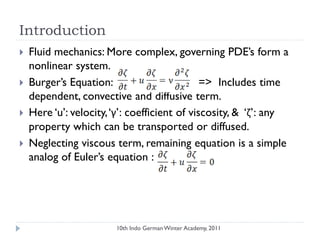
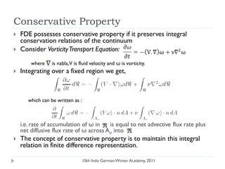
Fundamentals of Finite Difference Methods

Fundamentals of Finite Difference
Methods
Ashish Ranjan Jha, Electrical Engineering, IIT Roorkee
10th Indo German Winter Academy, 2011

Topics to be covered
 Introduction
 About PDEs(Partial Differential Equations)
 Various Discretization Methods
 FDM - Overview
 Basics of Finite Difference Methods
 Taylor Series Expansion
 Finite Difference Quotients
 Truncation Error
 Finite Difference Methods
 Explicit Method
 Implicit Method – Crank Nicholson Method
 Comparison of the two
 Consistency, Stability and Convergence
 Consistency
 Convergence
 Error and Stability Analysis –Von Neumann Analysis
 Application in Fluid Flow Equations
 Conservative property
 Transportive property
 Upwinding
 Hybrid Scheme

Introduction

About PDEs :
 A second order PDE :
 Linear Equations:A,B,C,D,E and F are constants or f(x,y)
 Non-linear Equations:A,B,C,D,E and F contain φ or its derivatives
 Quasilinear Equations: Important subclass of nonlinear equations.A,B,C,D,E and
F may be function of φ or its first derivatives
 Homogeneous: G=0
 Parabolic Equation: B*B - 4AC = 0
 Elliptic Equation: B*B – 4AC < 0
 Hyperbolic Equation: B*B – 4AC > 0

About PDEs :
 Some basic equations :
 Navier Stoke Equation : Elliptical in space ; Parabolic in time
 Laplace and Poisson Equations: Elliptic
 Fluid flow problems have non – linear terms called advection
and convection terms in momentum and energy equations
respectively.

Various Discretization Methods
 Finite Difference Method (FDM)
 Finite Element Method (FEM)
 FiniteVolume Method (FVM)
 Spectral Method
 Lattice Gas Cellular Automata (LGCA)

FDM - Overview
 Boundary Conditions
 No. of Boundary conditions required is order of highest
derivative appearing in each independent variable
 Unsteady equations governed by a first derivative in time
require initial condition to carry out the time integration
 Three types of spatial boundary conditions:
 Dirchlet Condition
 Neumann Condition
 Mixed Boundary Condition

FDM - Overview
 Basic Procedure
 Replace derivatives of governing equations with algebraic
difference quotients
 Results in a system of algebraic equations solvable for
dependent variables at discrete grid points
 Analytical solutions provide closed-form expressions –variation
of dependent variables in the domain
 Numerical solutions (finite difference) - values at discrete
points in the domain

FDM - Overview
 Discrete Grid Points
 Δx and Δy –spacing in positive
x and y direction
 Δx & Δy not necessarily uniform.
 In some cases, numerical
calculations performed on trans-
formed computational plane
having uniform spacing in transformed variables but
non uniform spacing in physical plane.
 Grid points identified by indices i and j in positive x and y
direction respectively.

Basics of Finite Difference Methods

Taylor Series Expansion
for small Δx higher order terms can be neglected.
n-order accurate Truncation error

Finite Difference Quotients and
Truncation Error
Forward Difference Truncation Error 𝒪(Δx)
Backward Difference Truncation Error 𝒪(Δx)
Central Difference Truncation Error 𝒪(Δx)2
Central Difference for Second Derivative

Finite Difference Quotients and
Truncation Error
 Basic concept: Replace each term of PDE with its finite
difference equivalent term
 Partial difference equation:
 Using Forward time Central Space (FTCS) method of
discretization:
 n: conditions at time t
 i: grid point in spatial dimension
 Truncation Error (TE) = 𝒪(Δt, (Δx)2)

Finite Difference Methods

Explicit Method
 Explicit method uses the fact that we know the
dependent variable, u at all x at time t from initial
conditions
 Since the equation contains only one unknown, (i.e. u
at time t+Δt), it can be obtained directly from known
values of u at t
 The solution takes the form of a “marching” procedure in
steps of time

Crank – Nicolson Implicit Method
 The unknown value u at time level (n+1) is expressed
both in terms of known quantities at n and unknown
quantities at (n+1).
 The spatial differences on RHS are expressed in terms of
averages between time level n and (n+1) :
 The above equation cannot result in a solution of at
grid point i.
 The eq. is written at all grid points resulting in a system of
algebraic equations which can be solved simultaneously
for u at all i at time level (n+1).

Crank – Nicolson Implicit Method
 The equation can be rearranged as
where r = αΔt/(Δx) 2
 On application of eq. at all grid points from i=1 to i=k+1 , the
system of eqs. with boundary conditions u=A at x=0 and u=D
at x=L can be expressed in the form of Ax = C
 A is the tridiagonal coefficient matrix and x is the solution
vector.The eq. can be solved using Thomas Algorithm

Explicit ~ Implicit – A Comparison
 Explicit Method
 Easy to set up.
 Constraint on mesh width, time-step.
 Less computer time.
 Implicit Method
 Complicated to set up.
 Larger computer time.
 No constraint on time step.
 Can be solved using Thomas Algorithm.

Consistency, Stability & Convergence

Consistency
 A finite difference representation of a PDE is said to be
consistent if:
 For equations where truncation error is 𝒪(Δx) or 𝒪(Δt)
or higher orders,TE vanishes as the mesh is refined
 However, for schemes where TE is 𝒪(Δt/Δx), the scheme
is not consistent unless mesh is refined in a manner such
that Δt/Δx→0
 For the Dufort-Frankel differencing scheme (1953), if
Δt/Δx does not tend to zero, a parabolic PDE may end up
as a hyperbolic equation

Convergence
 A solution of the algebraic equations that approximate a
PDE is convergent if the approximate solution approaches
the exact solution of the PDE for each value of the
independent variable as the grid spacing tends to zero :
RHS is the solution of algebraic equation

Errors & Stability Analysis
 Errors :
 A = Analytical solution of PDE
 D = Exact solution of finite difference equation
 N = Numerical solution from a real computer with finite
accuracy
 Discretization Error = A –D = Truncation error + error
introduced due to the treatment of boundary condition
 Round-off Error = ε= N –D
N = ε+ D
ε will be referred to as “error” henceforth

Errors & Stability Analysis
 Consider the 1-D unsteady state heat conduction equation and its FDE :
 N must satisfy the finite difference equation :
 Also, D being the exact solution also satisfies FDE :
 Subtracting above 2 equations, we see that error ε also satisfies FDE :
 If errors εi‟s shrink or remain same from step n to n+1, solution is stable.
Condition for stability is :

Application in Fluid Flow Equations

Introduction
 Fluid mechanics: More complex, governing PDE‟s form a
nonlinear system.
 Burger‟s Equation: => Includes time
dependent, convective and diffusive term.
 Here „u‟: velocity,„γ‟: coefficient of viscosity, & „ζ‟: any
property which can be transported or diffused.
 Neglecting viscous term, remaining equation is a simple
analog of Euler‟s equation :

Conservative Property
 FDE possesses conservative property if it preserves integral
conservation relations of the continuum
 Consider VorticityTransport Equation:
where is nabla,V is fluid velocity and ω is vorticity.
 Integrating over a fixed region we get,
which can be written as :
i.e. rate of accumulation of ω in is equal to net advective flux rate plus
net diffusive flux rate of ω across Ao into
 The concept of conservative property is to maintain this integral
relation in finite difference representation.

Conservative Property
 Consider inviscid Burger‟s equation :
 Evaluating the integral over a region running from i=I1
to i=I2 :
Thus, the FDE analogous to inviscid part of the
integral has preserved the conservative property.
 For non-conservative form of inviscid Burger‟s equation:
i.e. FDE analog has failed to preserve the conservative property
FDE Analog

Transportive Property
 FDE formulation of a flow is said to possess the transportive property if
the effect of perturbation is convected only in the direction of velocity
 Consider model Burger‟s equation in conservative form and a perturbation
εm = δ in ζ for u>0, all other ε=0
 Using FTCS, we find the transportive property to be violated
 On the contrary when an upwind scheme is used,
 => Downstream Location (m+1)

 => Point m of disturbance
 => Upstream Location (m-1)
 Upwind method maintains unidirectional flow of information.

The Upwind Method
 The inviscid Burger‟s equation in the following forms are
unconditionally unstable :
 The equations can be made stable by using backward space
difference scheme if u > 0 and forward space difference
scheme if u < 0 :
 Upwind method of discretization is necessary in convection
dominated flows.

References
 Knabner P., Angerman L. - “Numerical Methods for Elliptic
and Parabolic Partial Differential Equations”
 "Numerical simulation in fluid dynamics: a practical
introduction" by Michael Griebel, Thomas Dornseifer, Tilman
Neunhoeffe
 http://www10.informatik.uni-
erlangen.de/en/Teaching/Courses/WS2011/SiWiR/material/scri
pt.pdf
 "Introduction to Partial Differential Equations (A
ComputationalApproach)" by Aslak Tveito, Ragnar Winther
(Publisher: Springer Berlin)
 “Finite Difference Schemes and Partial Differential
Equations, Second Edition” , John C. Strikwerda

Fundamentals of Finite Difference Methods

More Related Content

What's hot

Similar to Fundamentals of Finite Difference Methods

Recently uploaded

Fundamentals of Finite Difference Methods