Downloaded 124 times
![Basic Steps in the Finite Element Method
Time Independent Problems
- Domain Discretization
- Select Element Type (Shape and Approximation)
- Derive Element Equations (Variational and Energy Methods)
- Assemble Element Equations to Form Global System
[K]{U} = {F}
[K] = Stiffness or Property Matrix
{U} = Nodal Displacement Vector
{F} = Nodal Force Vector
- Incorporate Boundary and Initial Conditions
- Solve Assembled System of Equations for Unknown Nodal
Displacements and Secondary Unknowns of Stress and Strain Values](https://image.slidesharecdn.com/femlecture-150828033122-lva1-app6892/85/Fem-lecture-10-320.jpg)
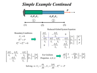
![Simple Element Equation Example
Direct Stiffness Derivation
1 2
k
u1 u2
F1 F2
}{}]{[
rmMatrix Foinor
2NodeatmEquilibriu
1NodeatmEquilibriu
2
1
2
1
212
211
FuK
F
F
u
u
kk
kk
kukuF
kukuF
=
=
−
−
+−=⇒
−=⇒
Stiffness Matrix Nodal Force Vector](https://image.slidesharecdn.com/femlecture-150828033122-lva1-app6892/85/Fem-lecture-17-320.jpg)
![One-Dimensional Bar Element
⇒δ++=δσ ∫∫ ΩΩ
udVfuPuPedV jjii
}]{[:LawStrain-Stress
}]{[}{
][
)(:Strain
}{][)(:ionApproximat
dB
dBd
N
dN
EEe
dx
d
ux
dx
d
dx
du
e
uxu
k
kk
k
kk
==σ
==ψ==
=ψ=
∑
∑
⇒+
= ∫∫
L
TT
j
iT
L
TT
fdxA
P
P
dxEA
00
][}{}{}{][][}{ NδdδddBBδd
∫∫ +=
L
T
L
T
fdxAdxEA
00
][}{}{][][ NPdBB
VectorentDisplacemNodal}{
VectorLoading][}{
MatrixStiffness][][][
0
0
=
=
=+
=
==
∫
∫
j
i
L
T
j
i
L
T
u
u
fdxA
P
P
dxEAK
d
NF
BB
}{}]{[ FdK =](https://image.slidesharecdn.com/femlecture-150828033122-lva1-app6892/85/Fem-lecture-19-320.jpg)
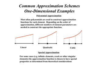
![Linear Approximation Scheme
[ ]
VectorentDisplacemNodal}{
MatrixFunctionionApproximat][
}]{[1
)()(
1
2
1
2
1
21
2211
21
12
1
212
11
21
=
=
=
−=
ψψ=
ψ+ψ=
+
−=
−
+=⇒
+=
=
⇒+=
d
N
dN
ntDisplacemeElasticeApproximat
u
u
L
x
L
x
u
u
u
uxux
u
L
x
u
L
x
x
L
uu
uu
Laau
au
xaau
x (local coordinate system)
(1) (2)
iu ju
L
x
(1) (2)
u(x)
x
(1) (2)
ψ1(x) ψ2(x)
1
ψk(x) – Lagrange Interpolation Functions](https://image.slidesharecdn.com/femlecture-150828033122-lva1-app6892/85/Fem-lecture-21-320.jpg)
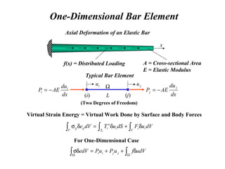
![Element Equation
Linear Approximation Scheme, Constant Properties
VectorentDisplacemNodal}{
1
1
2
][}{
11
1111
1
1
][][][][][
2
1
2
1
0
2
1
0
2
1
00
=
=
+
=
−
+
=+
=
−
−
=
−
−
===
∫∫
∫∫
u
u
LAf
P
P
dx
L
x
L
x
Af
P
P
fdxA
P
P
L
AE
L
LL
L
LAEdxAEdxEAK
o
L
o
L
T
L
T
L
T
d
NF
BBBB
+
=
−
−
⇒=
1
1
211
11
}{}]{[
2
1
2
1 LAf
P
P
u
u
L
AE o
FdK](https://image.slidesharecdn.com/femlecture-150828033122-lva1-app6892/85/Fem-lecture-22-320.jpg)
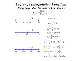
![Quadratic Approximation Scheme
[ ] }]{[
)()()(
42
3
2
1
321
332211
2
3213
2
3212
11
2
321
dN
ntDisplacemeElasticeApproximat
=
ψψψ=
ψ+ψ+ψ=
++=
++=
=
⇒++=
u
u
u
u
uxuxuxu
LaLaau
L
a
L
aau
au
xaxaau
x
(1) (3)
1u 3u
(2)
2u
L
u(x)
x
(1) (3)(2)
x
(1) (3)(2)
1
ψ1(x) ψ3(x)
ψ2(x)
=
−
−−
−
3
2
1
3
2
1
781
8168
187
3
F
F
F
u
u
u
L
AE
EquationElement](https://image.slidesharecdn.com/femlecture-150828033122-lva1-app6892/85/Fem-lecture-23-320.jpg)
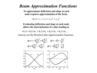
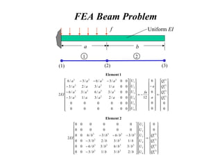
![One-Dimensional Beam Element
Deflection of an Elastic Beam
2
2423
1
1211
2
2
2
4
2
2
2
3
1
2
2
2
1
2
2
1
,,,
,
,
dx
dw
uwu
dx
dw
uwu
dx
wd
EIQ
dx
wd
EI
dx
d
Q
dx
wd
EIQ
dx
wd
EI
dx
d
Q
−=θ==−=θ==
−=
−=
=
=
I = Section Moment of Inertia
E = Elastic Modulus
f(x) = Distributed Loading
Ω
(1) (2)
Typical Beam Element
1w
L
2w
1θ 2θ
1M 2M
1V 2V
x
Virtual Strain Energy = Virtual Work Done by Surface and Body Forces
⇒δ++++=δσ ∫∫ ΩΩ
wdVfwQuQuQuQedV 44332211
∫∫ ++++=
L
T
L
dVfwQuQuQuQdxEI
0
44332211
0
][}{][][ NdBB T
(Four Degrees of Freedom)](https://image.slidesharecdn.com/femlecture-150828033122-lva1-app6892/85/Fem-lecture-27-320.jpg)
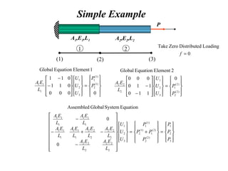
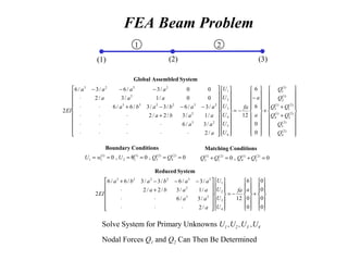
![Beam Element Equation
∫∫ ++++=
L
T
L
dVfwQuQuQuQdxEI
0
44332211
0
][}{][][ NdBB T
=
4
3
2
1
}{
u
u
u
u
d ][
][
][ 4321
dx
d
dx
d
dx
d
dx
d
dx
d φφφφ
==
N
B
−
−
−
−−−
== ∫
22
22
30
233
3636
323
3636
2
][][][
LLLL
LL
LLLL
LL
L
EI
dxEI
L
BBK T
−
+
=
−
−
−
−−−
L
LfL
Q
Q
Q
Q
u
u
u
u
LLLL
LL
LLLL
LL
L
EI
6
6
12
233
3636
323
3636
2
4
3
2
1
4
3
2
1
22
22
3
−
=
φ
φ
φ
φ
= ∫∫
L
LfL
dxfdxf
LL
T
6
6
12
][
0
4
3
2
1
0
N](https://image.slidesharecdn.com/femlecture-150828033122-lva1-app6892/85/Fem-lecture-29-320.jpg)

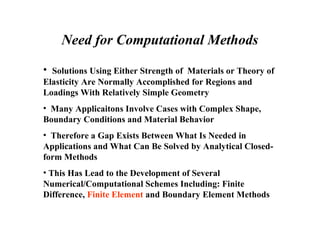
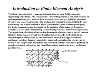
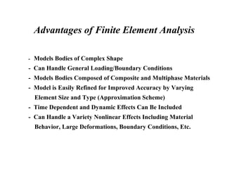
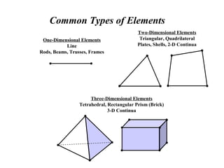
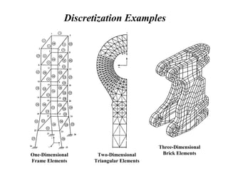
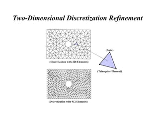
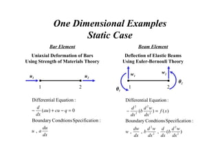
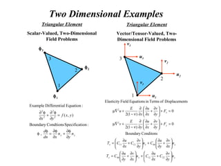
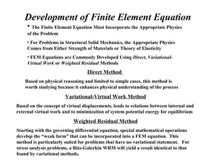
The document provides an introduction to finite element analysis. It discusses the need for computational methods to solve problems involving complex geometries and boundary conditions that cannot be solved through closed-form analytical methods. The finite element method is introduced as a numerical technique that involves discretizing a continuous domain into discrete subdomains called elements, and approximating variations in dependent variables within each element. This allows setting up algebraic equations that can be solved to approximate the continuous solution. Advantages of the finite element method include its ability to model complex shapes and behaviors, and refine solutions through mesh refinement. Basic concepts such as element types, discretization, and derivation of element equations are described.