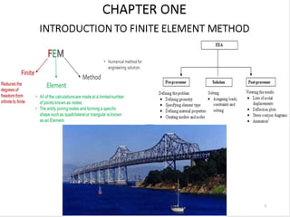
This document serves as an introduction to the finite element method (FEM), covering its background, applications, and key steps in its application. FEM is a numerical technique for solving engineering and mathematical physics problems, particularly those governed by boundary value problems. The document outlines the advantages of FEM, the role of computers in its execution, and various methods used to derive finite element equations.

1. 1
MIZAN-TEPI UNIVERSITY
COLLEGE OF ENGINEERING AND TECHNOLOGY
DEPARTMENT OF MECHANICAL ENGINEERING
Introduction to finite element method (FEM)
OR Finite Element Analysis (FEA)
Course code: MEng 4271
Course Title: Finite Element Method
Degree Program: BSc in Mechanical Engineering
Module: Advanced Design and Analysis

2. 2

3. 3
Learning Objectives
• To present an introduction to the finite element method
• To provide a brief history of the finite element method
• To describe the role of the computer in the development of
the finite element method
• To present the general steps used in the finite element
method
• To illustrate the various types of elements used in the finite
element method
• To show typical applications of the finite element method
• To summarize some of the advantages of the finite element
method

4. 4
Introduction to FEM
• The finite element method is a numerical method for solving
problems of engineering and mathematical physics.
• It is a numerical technique to obtain an approximate
solution to a class of problems governed by elliptic partial
differential equations.
• Such problems are called as boundary value problems(BVP)
as they consist of a partial differential equation and the
boundary conditions.
• A boundary value problem is a differential equation (or
system of differential equations) to be solved in a domain on
whose boundary a set of conditions is known.

5. 5
Introduction to FEM
Analytical solutions are those given by a mathematical
expression that yields the values of the desired unknown
quantities at any location in a body and are thus valid for an
infinite number of locations in the body
These analytical solutions generally require the solution of
ordinary or partial differential equations, which, because
of the complicated geometries, loadings, and material
properties, are not usually obtainable
Hence we need to rely on numerical methods, such as the
FEM, for acceptable solutions
FEM results in a system of simultaneous algebraic equations
for solution, rather than requiring the solution of
differential equations

6. 6
Introduction FEM
The goal of this procedure is to transform the differential
equations into a set of linear equations, which can then be
solved by the computer in a routine manner
Hence this process of modeling a body by dividing it into an
equivalent system of smaller bodies or units (finite
elements) interconnected at points common to two or
more elements (nodal points or nodes) and/or boundary
lines and/or surfaces is called discretization

7. 7
Introduction FEM
In the finite element method, instead of solving the problem
for the entire body in one operation, we formulate the
equations for each finite element and combine them to
obtain the solution of the whole body.
Briefly, the solution for structural problems typically refers to
determining the displacements at each node and the
stresses within each element making up the structure that
is subjected to applied loads.
In nonstructural problems, the nodal unknowns may, for
instance, may be temperatures or fluid pressures due to
thermal or fluid fluxes.

8. 8
Background of FEM
1940s - Modern development of FEM began in the field of
structural engineering.
1950s - The development of high-speed digital computers
made possible FEM equations to be expressed in matrix
notation.
Early1960s – FEM was extended to three-dimensional
problems. (small strain, small/large displacements, elastic
and non-linear material behavior, buckling problems).
In 1965 Archer developed method for dynamic analysis.
Late1960s - FEM had been applied to nonstructural
applications such as fluid flow, and heat conduction.

9. 9
Introduction FEM
Typical structural areas include,
1. Stress analysis, including
a. Truss and frame analysis, and
b. Stress concentration problems typically associated
with holes, fillets, or
c. Other changes in geometry in a body
2. Buckling
3. Vibration analysis

10. 10
Applications of the FEM
Nonstructural problems include
1. Heat transfer
2. Fluid flow, including seepage through porous media
3. Distribution of electric or magnetic potential
Finally, some biomechanical engineering problems typically
include
1. Analyses of human spine,
2. skull, hip joints,
3. jaw/gum tooth implants,
4. heart, and eye

11. 11
Introduction to Matrix Notation
• Matrix notation represents a simple system for writing and
solving sets of simultaneous algebraic equations.
• Matrix – a rectangular array of quantities arranged in rows
and columns that is used to express and solve a system of
equations.
• A rectangular matrix is indicated by square bracket notation
[ ].
• A column matrix is indicated by brace notation { }

12. 12
Column matrices
The column matrices represent the force components {F}
acting at various nodes or points (1,2…..,n) on a structure and
the corresponding set of nodal displacements {d}
Notation: Subscripts to the right of F identify the node and
direction of force, respectively. The x, y, and z displacements
at a node are denoted by u, v, and w.

13. 13
Rectangular matrices
• Here are square matrices, a type of rectangular matrices.
• The first [k] is the element stiffness matrix and the second
[K] is the global stiffness matrix

14. 14
Global Stiffness Equation
The above equation is called the global stiffness equation and
represents a set of simultaneous equations
This equation can be expanded into matrix form:

15. 15
Role of the Computer
• With the development of computers in the 1950s, the finite
element method became a practical tool of analysis
• With modern computers computational programs with
millions of unknowns can be solved
• To use the computer, the analyst, having defined the finite
element model, inputs the information for calculation
• The information may include the position of the elemental
nodal coordinates, material properties, the applied load,
boundary conditions, or constraints
• The computer then generates and solves the equations
and outputs results for interpretation

16. 16
Primary Methods Used to Derive the Finite Element
Equations
(1) Direct approach,
(2) Variation approach,
(3) Energy approach and
(4) Weighted residual approach.

17. 17
Direct Methods
Simplest methods and yield a clear physical insight into the
finite element method
• Limited in its application to one-dimensional elements
• There are two general direct approaches:
The force or flexibility method which uses internal forces
as the unknowns to the problems
The displacement or stiffness method which assumes the
displacement of the nodes as the unknowns of the problem
• For computational purposes, the displacement method is
more desirable and is more widely used

18. 18
Variation Methods
• Easier to use for deriving finite element equations
for two- and three-dimensional elements when compared to
the direct methods
• Requires the existence of a functional, that upon minimizing
yields the stiffness matrix and related element equations
• For structural/stress analysis problems, the principle of
minimum potential energy is used as the functional

19. 19
Weighted Residual Methods
• Allow the finite element method to be applied directly to
any differential equation without a variation principle
• A very well-known weighted residual method is the Galerkin
method, for deriving the bar element stiffness matrix and
associated element equations

20. 20
General Steps of the Finite Element Method
Step 1 - Discretize and Select Element Types
Step 2 - Select a Displacement Function
Step 3 - Define the Strain/Displacement and Stress/Strain
Relationships
Step 4 - Derive the Element Stiffness Matrix and Equations
Step 5 - Assemble the Element Equations and Introduce
Boundary Conditions
Step 6 - Solve for the Unknown Degrees of Freedom (or
Generalized Displacements)
Step 7 - Solve for the Element Strains and Stresses
Step 8 - Interpret the Results

21. 21
General Steps of the Finite Element Method
The analyst must make decisions regarding:
• Dividing the structure or continuum into finite
elements
• The element type or types to be used in the analysis
• The kinds of loads to be applied
• The types of boundary conditions or supports to be applied
• The other steps, 2 through 7, are carried out automatically
by a computer program

22. 22
Step 1: Discretize and Select the Element Types
• The total number of elements used and their variation in
size and type are matters of engineering judgment.
• Elements must be made small enough to give usable results
and yet large enough to reduce computational effort.
• The discretized body or mesh is often created with mesh-
generation programs

23. 23
Element Types

24. 24
Element Types

25. 25
Step 2: Select a Displacement Function
The function is defined within the element using the nodal
values of the elements.
• Linear, quadratic, and cubic polynomials are frequently used
functions
• Trigonometric series can also be used
• The continuous quantity, such as the displacement
throughout the body, is approximated by a discrete model
composed of piecewise-continuous functions

26. 26
Step 3: Define the Element Relationships
• The relationships are necessary for deriving the equations
for each finite element
• In the case of structural stress analysis problems, the
strain/displacement and stress/stress relationships must be
defined
=
• The ability to define the material behavior accurately is most
important in obtaining acceptable results

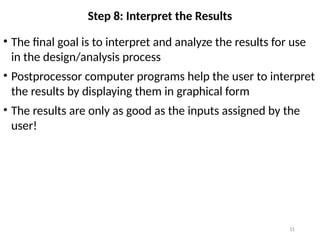
27. 27
Step 4: Derive the Element Stiffness Matrix Equations
• These equations can be written in matrix form as:
• Or in compact matrix form as
Where {f} is the vector of element nodal forces, [k] is the
element stiffness matrix, and {d} is the vector of unknown
element nodal degrees of freedom

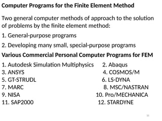
28. 28
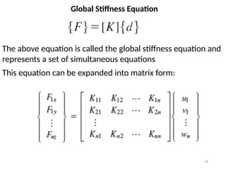
Step 5: Assemble the Element Equations
• The individual element nodal equilibrium equations
generated in step 4 are assembled into the global nodal
equilibrium equations
• The final assembled or global equation is written in matrix
form as:
• Where {F} is the vector of global nodal forces, [K] is the
structure global stiffness matrix, and {d} is now the vector of
known and unknown structure nodal degree of freedom
• Boundary conditions must be invoked to remove the
singularity problem of the global stiffness matrix [K]

29. 29
Step 6: Solve for the Unknown Degrees of Freedom
• A set of simultaneous algebraic equations, accounting for
the boundary conditions, can be written in expanded matrix
form as:
• Where n is now the structure total number of unknown
nodal degrees of freedom
• These equations are then solved for the ds, called the
primary unknowns, using an elimination or iterative method

30. 30
Step 7: Solve for the Element Secondary Quantities
• The secondary quantities are those that can be directly
expressed in terms of the calculated degrees of freedom
from Step 6
• For the structural stress-analysis problems, the important
secondary quantities are stress and strain or moment and
shear forces

31. 31
Step 8: Interpret the Results
• The final goal is to interpret and analyze the results for use
in the design/analysis process
• Postprocessor computer programs help the user to interpret
the results by displaying them in graphical form
• The results are only as good as the inputs assigned by the
user!

32. 32
Applications of the Finite Element Method
Typical structural areas include:
• Stress analysis and stress concentration problems
• Analysis of human spine, skull, hip, etc…
• Buckling, such as in columns or frames
• Vibration analysis
• Impact problems

33. 33
Applications of the Finite Element Method
Nonstructural problems include:
• Heat transfer such as in electronic devices and cooling fins
• Fluid flow including seepage through porous media, air flow
around race cars, or cooling ponds
• Distribution of electric or magnetic potential, such as in
antennas and transistors

34. 34
Advantages of the Finite Element Method
The ability to:
1. Model irregularly shaped bodies quite easily
2. Handle general load conditions without difficulty
3. Model bodies composed of several different materials
4. Handle virtually unlimited numbers and kinds of boundary
conditions
5. Vary the size of the elements
6. Alter the finite element model relatively easily and cheaply
7. Include dynamic effects
8. Handle nonlinear behavior

35. 35
Computer Programs for the Finite Element Method
Two general computer methods of approach to the solution
of problems by the finite element method:
1. General-purpose programs
2. Developing many small, special-purpose programs
Various Commercial Personal Computer Programs for FEM
1. Autodesk Simulation Multiphysics 2. Abaqus
3. ANSYS 4. COSMOS/M
5. GT-STRUDL 6. LS-DYNA
7. MARC 8. MSC/NASTRAN
9. NISA 10. Pro/MECHANICA
11. SAP2000 12. STARDYNE

36. 36
What is Modeling ?
- Modeling and simulation (M&S) is the use of a physical or
logical representation of a given system to generate data and
help determine decisions or make predictions about the
system.
- M&S is widely used in the social and physical sciences,
engineering, manufacturing and product development, among
many other areas.
- A Representation of an object, a system, or an idea in some
form other than that of the entity itself.
- This implies that a model can be used to answer questions
about a system without doing experiments on the real system

37. 37
Why is modeling required?
Modeling may be quite useful:
– To gauge the mass of the Earth, not using any balance
– To quantify the amount of blood inside a living human body
– To predict the population of China for the year 2050
– To assess the impact of 30% reduction in income tax over
the national economy
– To find the temperature at the surface or at the center of
the sun
– Crush Analysis of vehicle
– To determine the mean time between failures (MTBF) or
average life span of an electric bulb etc...

38. 38
General scenario of Modeling a physical problem

39. 39
Mathematical Model
A mathematical model is a mathematical description of
properties and interactions in the system
The development of a mathematical model depends on:
• The system boundary, system components, material
property and their interactions
• Type of analysis that we want to perform, like steady
state or transient analysis
• Assumptions that we will consider while model
development

40. 40
Computational Models
• Procedures of formulating and solving Engineering problems
• Broadly speaking, require simulation to reveal their
behaviors. Whereas the behavior of mathematical models can
be revealed by the application of analytical techniques
• Computational models involve either a large system of
equations and/or an algorithmic component
• Computational Modelling uses numerical Technique to solve
problems
– Finite difference Method
– Finite Element Method
– Finite Volume Method

41. 41
Processes leading to fabrication of advanced engineering
systems

42. 42
The End Of Chapter Two
Thank You
Any Question ??????