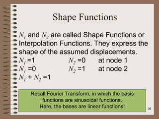
Downloaded 93 times
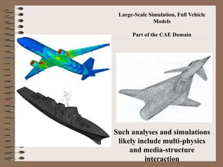
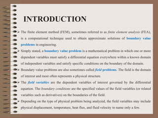
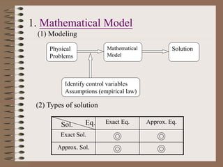
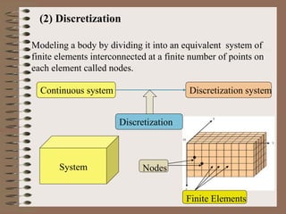

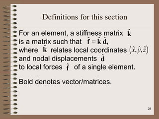
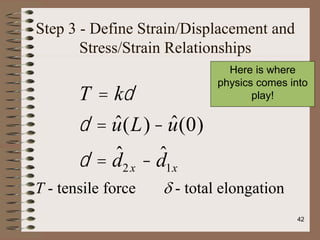
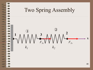
![Step 2 - Select a Displacement Function
Assume a displacement function
Assume a linear function.
Number of coefficients = number of d-o-f
Write in matrix form.
û
û = a1 + a2x̂
û = 1 x̂
[ ]
a1
a2
ì
í
î
ü
ý
þ
34](https://image.slidesharecdn.com/femchapter1-211118120512/85/Finite-element-method-34-320.jpg)
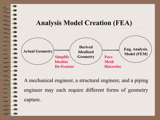
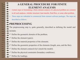
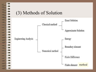
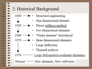
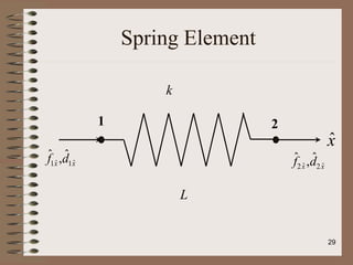
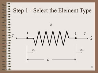
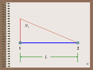
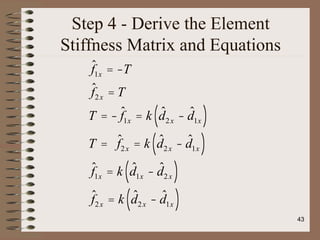
![In matrix form:
û = 1-
x̂
L
x̂
L
é
ë
ê
ù
û
ú
d̂1x
d̂2x
ì
í
ï
î
ï
ü
ý
ï
þ
ï
û = N1 N2
[ ]
d̂1x
d̂2x
ì
í
ï
î
ï
ü
ý
ï
þ
ï
Where :
N1 =1-
x̂
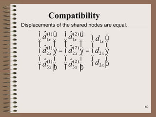
L
and N2 =
x̂
L
37](https://image.slidesharecdn.com/femchapter1-211118120512/85/Finite-element-method-37-320.jpg)
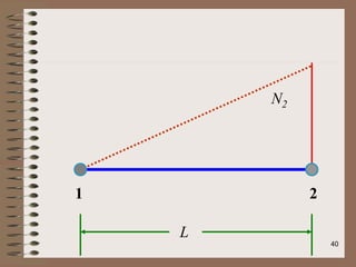
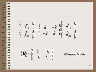
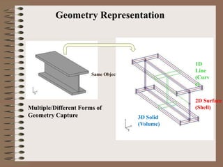
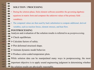
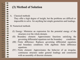
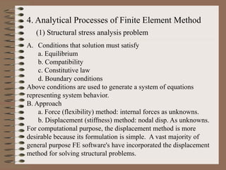
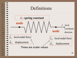
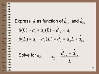
![Step 5 - Assemble the Element Equations to Obtain the
Global Equations and Introduce the B.C.
K
[ ] = k̂(e)
é
ë
ù
û
e=1
N
å
F
{ } = f̂(e)
{ }
e=1
N
å
Note: not simple addition!
An example later.
(e) indicates
“element” index
45](https://image.slidesharecdn.com/femchapter1-211118120512/85/Finite-element-method-45-320.jpg)
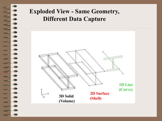
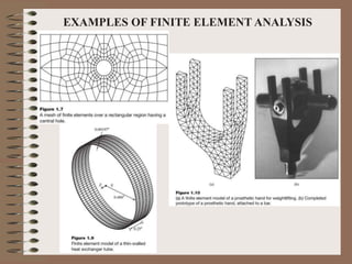
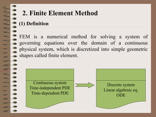
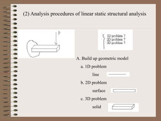
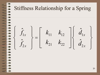
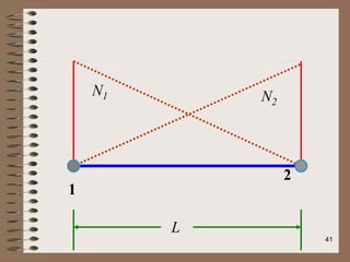
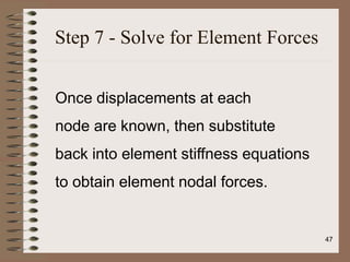
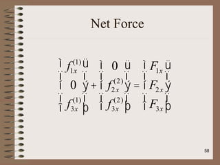
![Step 6 - Solve for Nodal
Displacements
Solve :
K
[ ] d
{ } = F
{ }
46](https://image.slidesharecdn.com/femchapter1-211118120512/85/Finite-element-method-46-320.jpg)
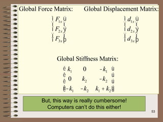
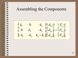
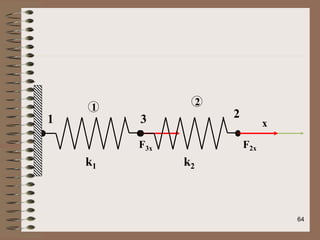
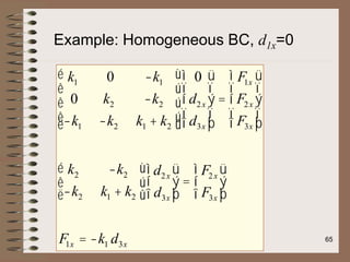
![F3x = -k1d1x + k1d3x + k2d3x - k2d2x
F2x = -k2d3x + k2d2x
F1x = k1d1x - k1d3x
In the matrix form:
F1x
F2x
F3x
ì
í
ï
î
ï
ü
ý
ï
þ
ï
=
k1 0 -k1
0 k2 -k2
-k1 -k2 k1 + k2
é
ë
ê
ê
ê
ù
û
ú
ú
ú
d1x
d2x
d3x
ì
í
ï
î
ï
ü
ý
ï
þ
ï
or
F
[ ]= K
[ ] d
{ }
Substitution will give
you these equations
52](https://image.slidesharecdn.com/femchapter1-211118120512/85/Finite-element-method-52-320.jpg)
![Assembly of [K] -
An Alternative Method
k1
1 2
k2
1
2
3 x
F3x F2x
54](https://image.slidesharecdn.com/femchapter1-211118120512/85/Finite-element-method-54-320.jpg)
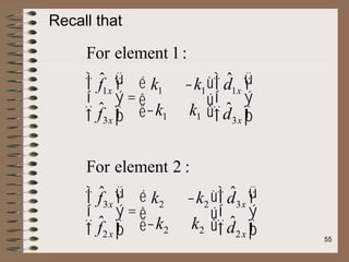
![Assembly of [K] - An
Alternative Method
node 1 3
[k(1)
] =
k1 -k1
-k1 k1
é
ë
ê
ê
ù
û
ú
ú
node 3 2
[k(2)
] =
k2 -k2
-k2 k2
é
ë
ê
ê
ù
û
ú
ú
Insert row and
column 2 with zeros
Flip row, flip
columns, and insert
row 1 with zeros
1
3
3
2
56](https://image.slidesharecdn.com/femchapter1-211118120512/85/Finite-element-method-56-320.jpg)
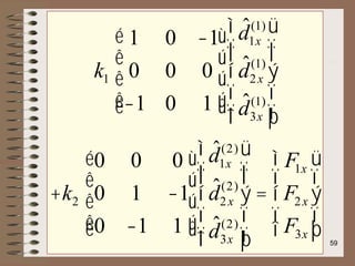
![Expand Local [k] matrices to
Global Size
k1
1 0 -1
0 0 0
-1 0 1
é
ë
ê
ê
ê
ù
û
ú
ú
ú
d̂1x
(1)
d̂2x
(1)
d̂3x
(1)
ì
í
ï
ï
î
ï
ï
ü
ý
ï
ï
þ
ï
ï
=
f1x
(1)
f2x
(1)
f3x
(1)
ì
í
ï
î
ï
ü
ý
ï
þ
ï
k2
0 0 0
0 1 -1
0 -1 1
é
ë
ê
ê
ê
ù
û
ú
ú
ú
d̂1x
(2)
d̂2x
(2)
d̂3x
(2)
ì
í
ï
ï
î
ï
ï
ü
ý
ï
ï
þ
ï
ï
=
f1x
(2)
f2x
(2)
f3x
(2)
ì
í
ï
î
ï
ü
ý
ï
þ
ï Computers
can do this!
57](https://image.slidesharecdn.com/femchapter1-211118120512/85/Finite-element-method-57-320.jpg)


The document provides an introduction to the finite element method (FEM). It discusses how FEM can be used to obtain approximate solutions to boundary value problems in engineering. It outlines the general steps involved, including preprocessing (defining the model), solution/processing (computing unknown values), and postprocessing (analyzing results). Examples of FEM applications include structural analysis, fluid flow, heat transfer, and more. The key aspects of FEM include discretizing the domain into simple elements, choosing shape functions to approximate variations within each element, and assembling the element equations into a global system of equations to solve.