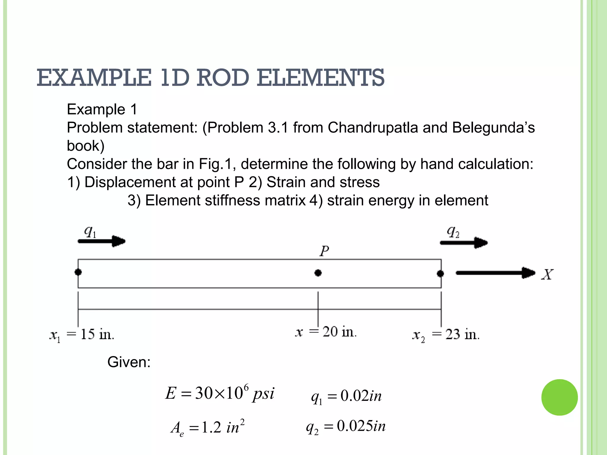
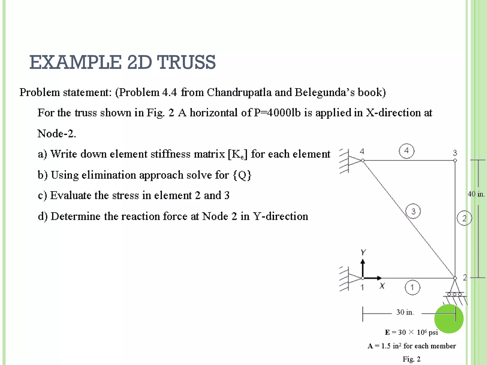
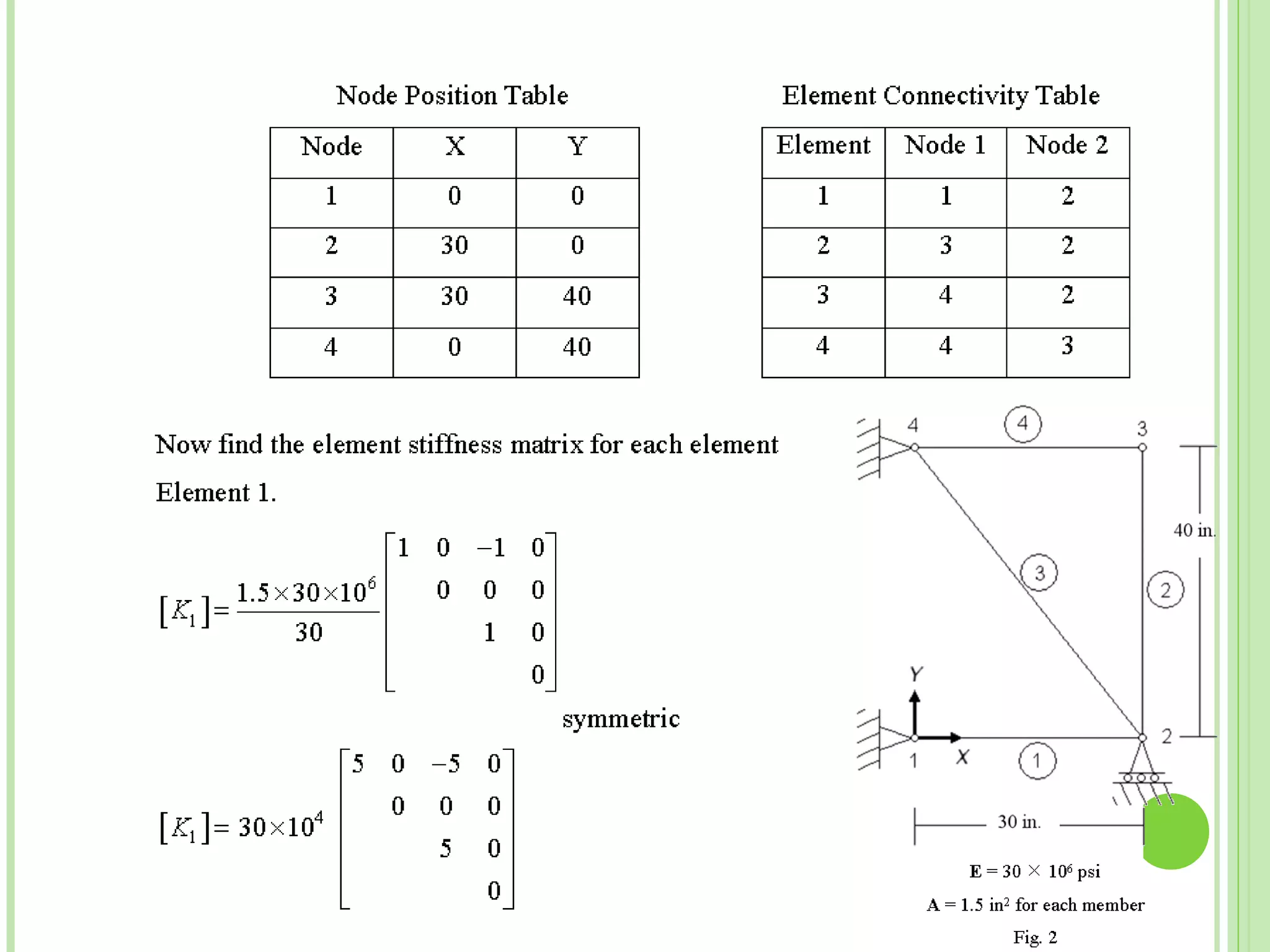
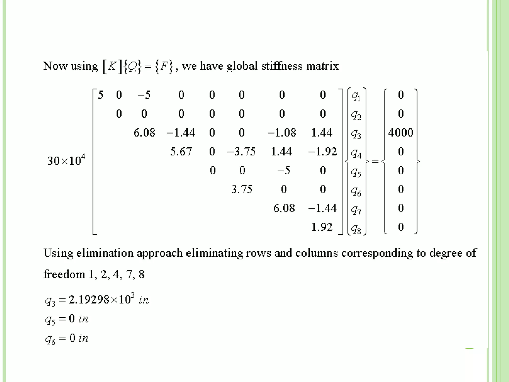
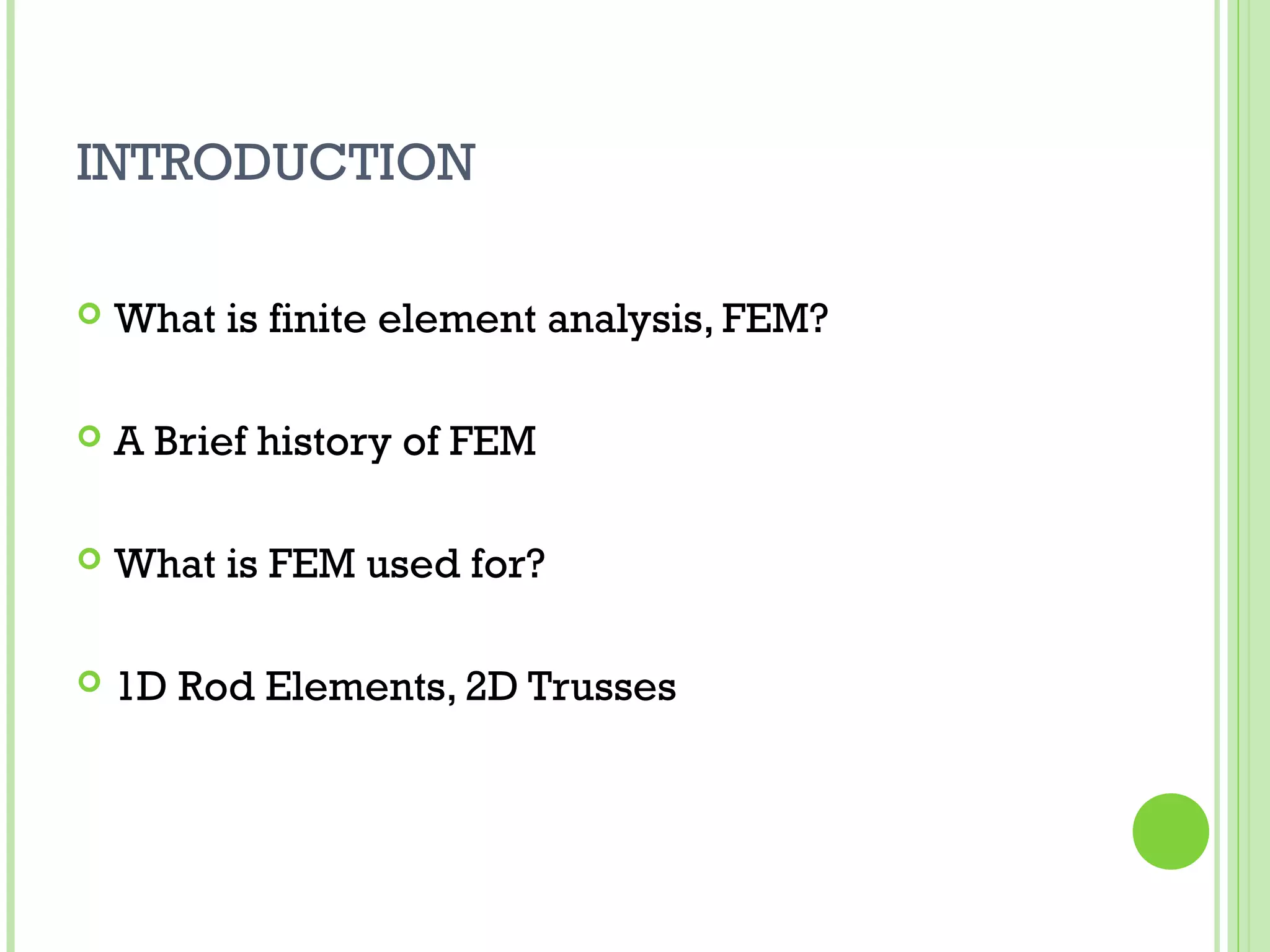
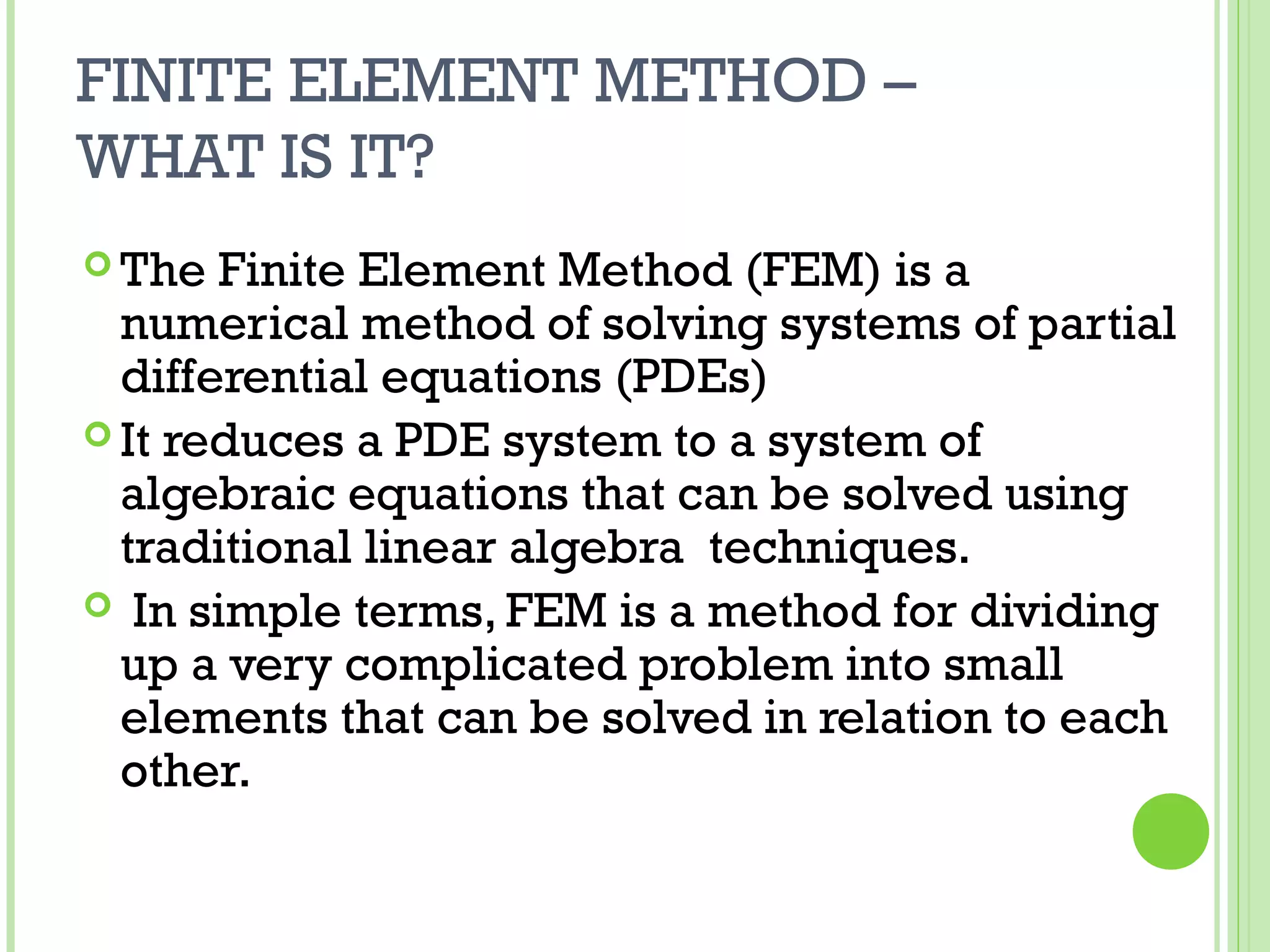
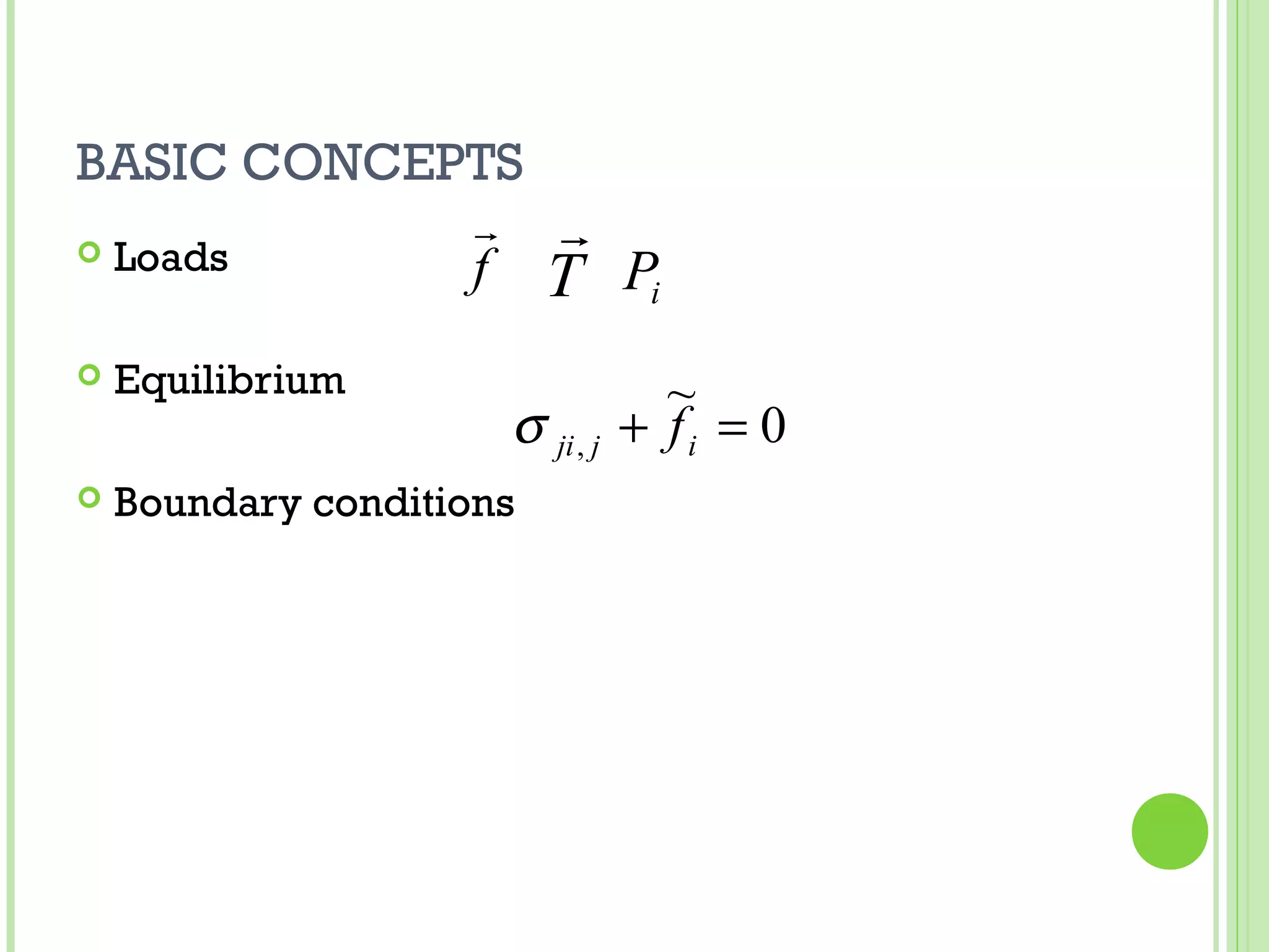
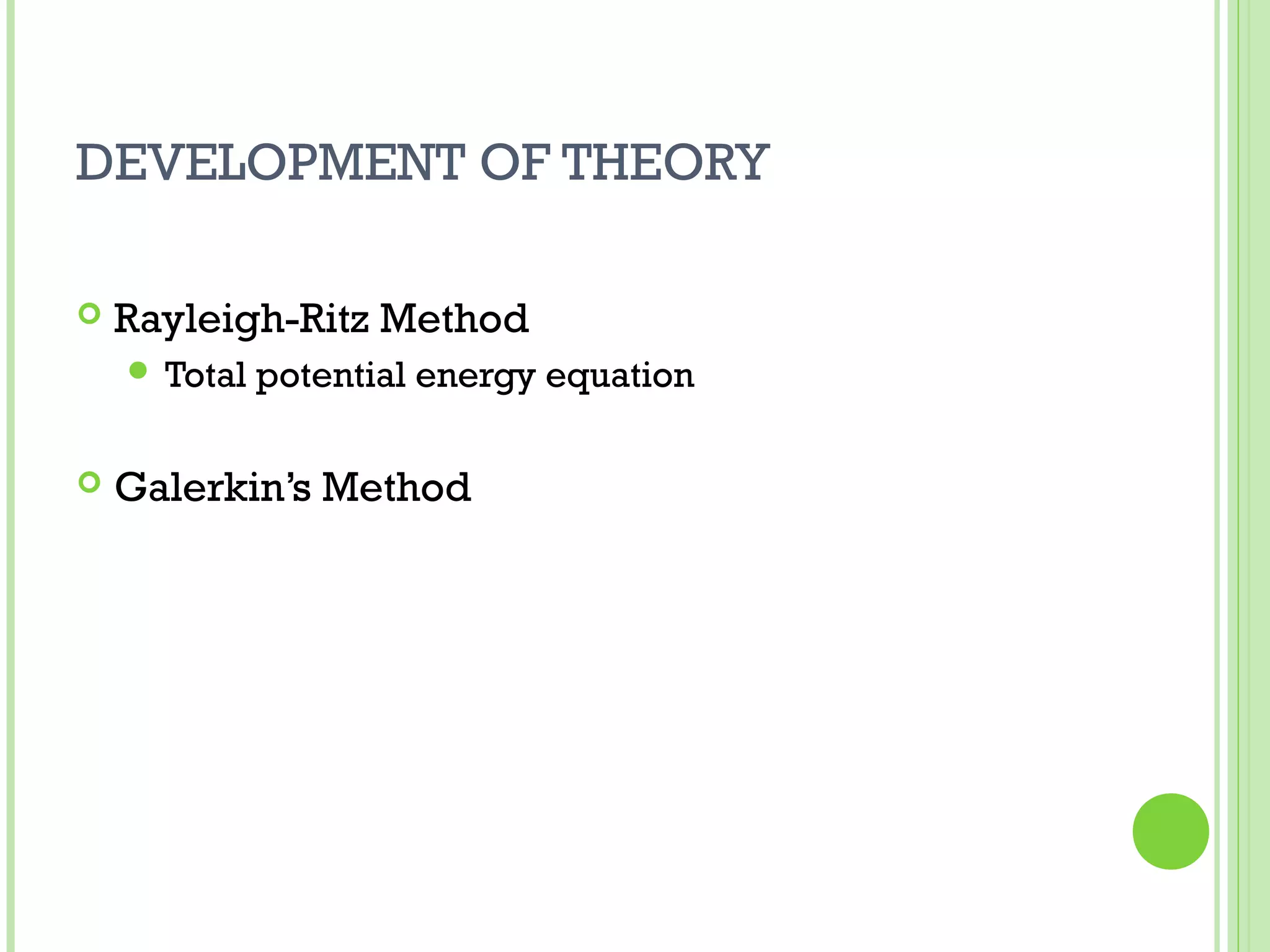
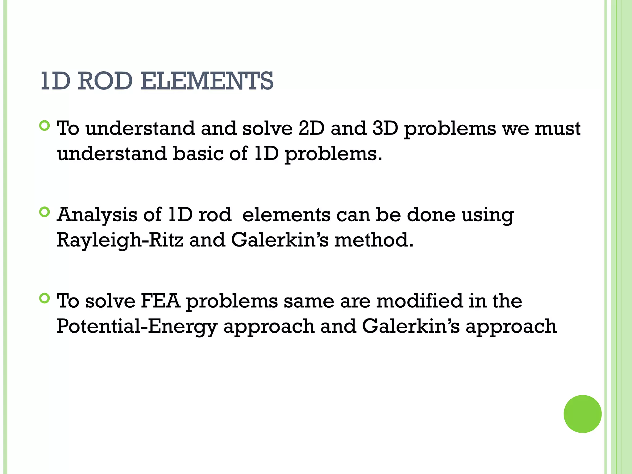
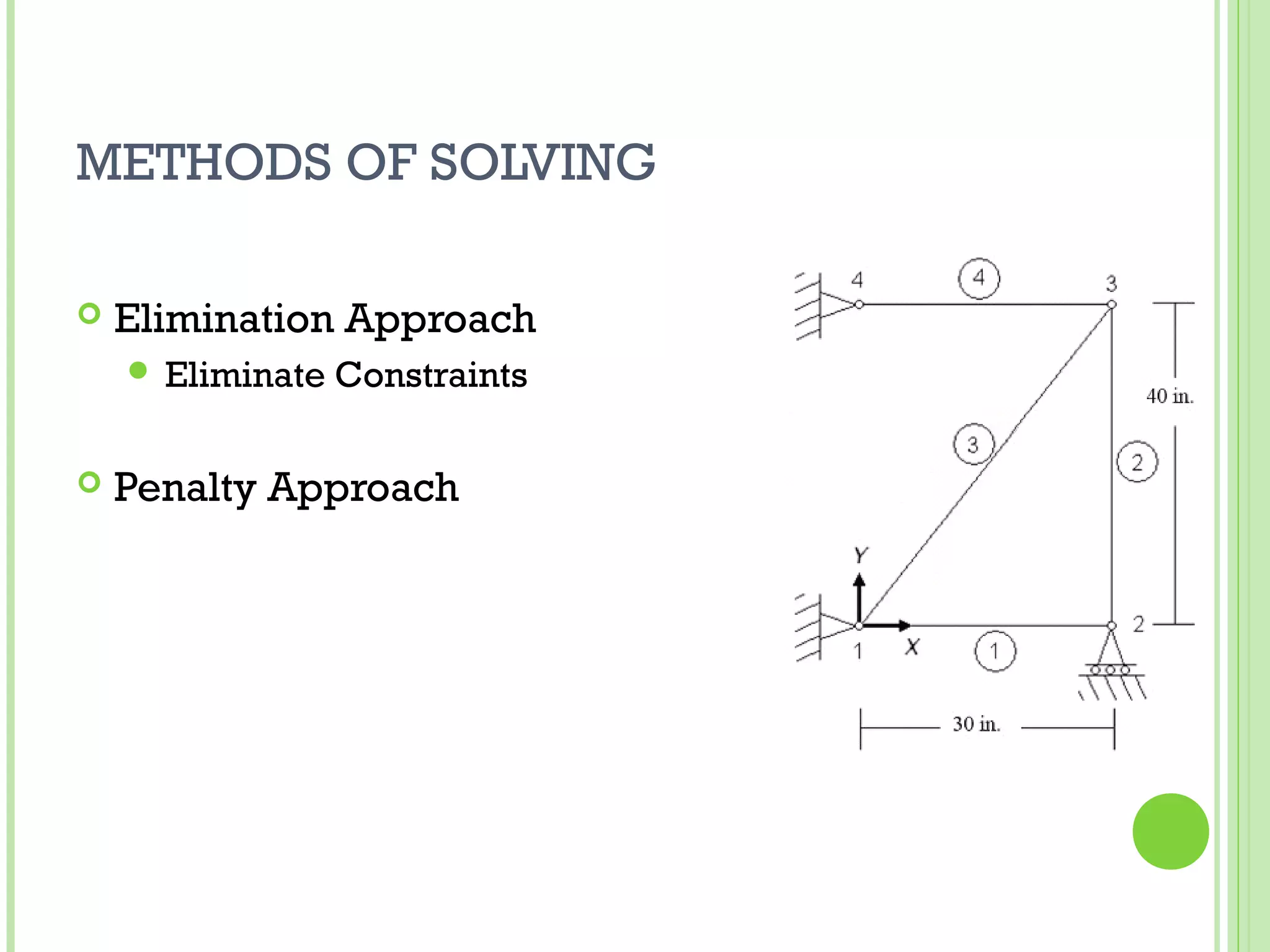
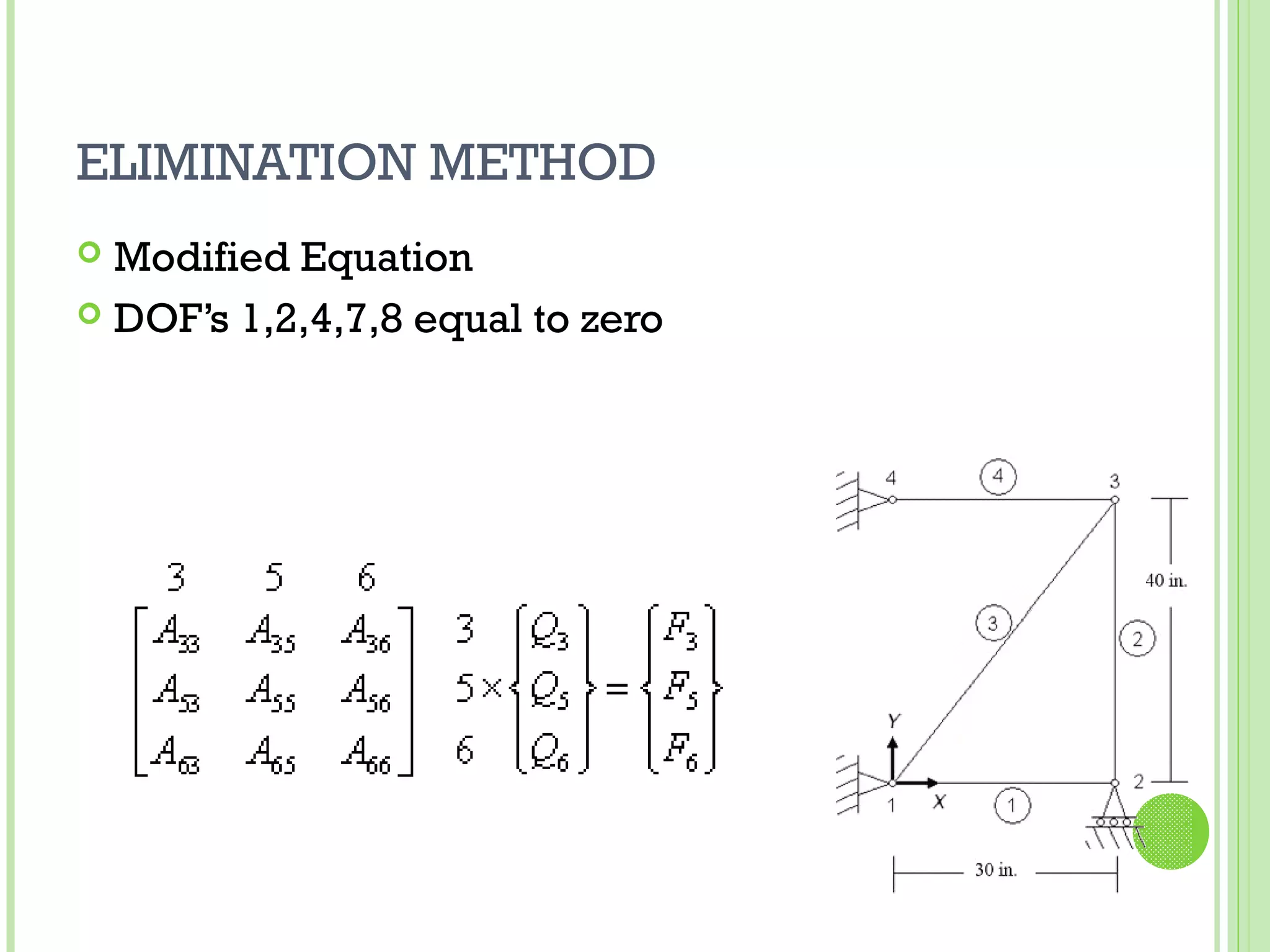
FINITE ELEMENT METHOD
INTRODUCTION

   What is finite element analysis, FEM?

   A Brief history of FEM

   What is FEM used for?

   1D Rod Elements, 2D Trusses
FINITE ELEMENT METHOD –
WHAT IS IT?
 The  Finite Element Method (FEM) is a
  numerical method of solving systems of partial
  differential equations (PDEs)
 It reduces a PDE system to a system of
  algebraic equations that can be solved using
  traditional linear algebra techniques.
  In simple terms, FEM is a method for dividing
  up a very complicated problem into small
  elements that can be solved in relation to each
  other.
Overview of the Finite
   Element Method

( S ) ⇔(W ) ≈ ( G ) ⇔( M )
Strong   Weak   Galerkin   Matrix
form     form   approx.    form
1. Lord John William Strutt Rayleigh (late 1800s), developed a
   method for predicting the first natural frequency of simple
   structures. It assumed a deformed shape for a structure and
   then quantified this shape by minimizing the distributed energy
   in the structure.

2. Ritz then exp Walter ended this into a method, now known as
   the Rayleigh-Ritz method, for predicting the stress and
   displacement behavior of structures.
3. Dr. Ray Clough coined the term “finite element” in 1960. The 1960s saw
   the true beginning of commercial FEA as digital computers replaced analog
   ones with the capability of thousands of operations per second.

4. In the 1950s, a team form Boeing demonstrated that complex surfaces
   could be analyzed with a matrix of triangular shapes.

5. In 1943, Richard Courant proposed breaking a continuous system into
   triangular segments. (The unveiling of ENIAC at the University of
   Pennsylvania.)
6. In the early 1960s, the MacNeal-Schwendle Corporation (MSC) develop a
   general purpose FEA code. This original code had a limit of 68,000
   degrees of freedom. When the NASA contract was complete, MSC
   continued development of its own version called MSC/NASTRAN, while the
   original NASTRAN become available to the public and formed the basis of
   dozens of the FEA packages available today. Around the time        6

   MSC/NASTRAN was released, ANSYS, MARC, and SAP were introduced.
7. By the 1970s, Computer-aided design, or CAD, was introduced later in the
decade.


8. standards such as IGES and DXF. Permitted limited geometry transfer
   between the systems.

9. In the 1980s,CAD progressed from a 2D drafting tool to a 3D surfacing tool,
   and then to a 3D sIn the 1980s, the use of FEA and CAD on the same
   workstation with developing geometry olid modeling system. Design
   engineers began to seriously consider incorporating FEA into the general
   product design process.

10. As the 1990s draw to a place, the PC platform has become a major force in
    high end analysis. The technology has become to accessible that it is
    actually being “hidden” inside CAD packages.
                                                                        7
BASIC CONCEPTS
 Loads
             
            f T Pi
   Equilibrium                    ~
                      σ ji , j   + fi = 0
   Boundary conditions
DEVELOPMENT OF THEORY

   Rayleigh-Ritz Method
     Total   potential energy equation

   Galerkin’s Method
1D ROD ELEMENTS
   To understand and solve 2D and 3D problems we must
    understand basic of 1D problems.

   Analysis of 1D rod elements can be done using
    Rayleigh-Ritz and Galerkin’s method.

   To solve FEA problems same are modified in the
    Potential-Energy approach and Galerkin’s approach
1D ROD ELEMENTS

   Loading consists of three types : body force f , traction
    force T, point load Pi


   Body force: distributed force , acting on every
    elemental volume of body i.e. self weight of body.

   Traction force: distributed force , acting on surface of
    body i.e. frictional resistance, viscous drag and surface
    shear

   Point load: a force acting on any single point of element
1D ROD ELEMENTS                       Element -1         Element-2

                                               1 T e 
   Element strain energy                 U e = q [k ]q
                                               2
   Element stiffness matrix
                                                E e Ae      1 − 1
                                         [k ] =
                                            e
                                                           − 1 1 
                                                  le             
   Load vectors
     Element body load vector
     Element traction-force vector              e Ae l e f   1
                                                f =            
                                                      2        1
                                                 e Tl e   1
                                                T =        
                                                     2     1
2D TRUSS
   2 DOF

   Transformations

   Modified Stiffness Matrix

   Methods of Solving
2D TRUSS

   Transformation Matrix
     Direction   Cosines

                            le =   ( x2 − x1 ) 2 + ( y 2 − y1 ) 2

                                          x 2 − x1
           l m 0 0          l = cos θ =
    [ L] =                                   le
            0 0 l m
                    
                                          y 2 − y1
                              m = sin θ =
                                              le
2D TRUSS

   Element Stiffness Matrix


                           l2    lm     − l 2 − lm 
                                                  2
                   E e Ae  lm   m2      − lm − m 
          [k e ] =
                     l e  − l 2 − lm     l2    lm 
                                                 2 
                          − lm − m
                                     2
                                         lm   m   
METHODS OF SOLVING

   Elimination Approach
     Eliminate   Constraints

   Penalty Approach
ELIMINATION METHOD
   Set defection at the constraint to equal zero
ELIMINATION METHOD
 Modified Equation
 DOF’s 1,2,4,7,8 equal to zero
2D TRUSS

   Element Stresses
                                 Ee                
                              σ=    [ − l − m l m] q
                                 le
   Element Reaction Forces

                                             
                                     R = [ K ]Q
2D TRUSS

   Development of Tables

     Coordinate Table
     Connectivity Table
     Direction   Cosines Table
2D TRUSS
   Coordinate Table
                      E.g;
2D TRUSS
   Connectivity Table
                        E.g;
2D TRUSS


le =   ( x2 − x1 ) 2 + ( y 2 − y1 ) 2
            x 2 − x1
l = cos θ =
                le
            y 2 − y1
m = sin θ =
                le
3D TRUSS STIFFNESS MATRIX
   3D Transformation Matrix
     Direction     Cosines


                                l m n 0 0 0
                        [ L] = 
                                0 0 0 l m n
                                            


               le =       ( x 2 − x1 ) 2 + ( y 2 − y1 ) 2 + ( z 2 − z1 ) 2
                    x 2 − x1                     y 2 − y1                       z 2 − z1
      l = cos θ =                 m = cos φ =                     n = cos ϕ =
                        le                           le                             le
3D TRUSS STIFFNESS MATRIX
   3D Stiffness Matrix


                         l2    lm   ln   − l 2 − lm − ln 
                                                         
                         lm    m2   mn − lm − m 2 − mn 
                 E e Ae  ln    mn   n2   − ln − mn − n 2 
        [k e ] =                                         
                   l e  − l 2 − lm − ln   l 2
                                                 lm   ln 
                        − lm − m 2 − mn lm     m2   mn 
                                                         
                         − ln − mn − n
                                        2              2
                                          ln   mn   n   
EXAMPLE 1D ROD ELEMENTS
  Example 1
  Problem statement: (Problem 3.1 from Chandrupatla and Belegunda’s
  book)
  Consider the bar in Fig.1, determine the following by hand calculation:
  1) Displacement at point P 2) Strain and stress
           3) Element stiffness matrix 4) strain energy in element


        Given:

                 E = 30 ×106 psi       q1 = 0.02in
                 Ae = 1.2 in 2        q2 = 0.025in
Solution:
1) Displacement (q) at point P
We have


Now linear shape functions N1( ) and N2( ) are given by

                      And
EXAMPLE 2D TRUSS
CONCLUSION

   Good at Hand Calculations, Powerful when
    applied to computers

   Only limitations are the computer limitations
MATLAB PROGRAM TRUSS2D.M
REFERENCES

Introduction to finite element method(fem)

  • 1.
  • 2.
    INTRODUCTION  What is finite element analysis, FEM?  A Brief history of FEM  What is FEM used for?  1D Rod Elements, 2D Trusses
  • 3.
    FINITE ELEMENT METHOD– WHAT IS IT?  The Finite Element Method (FEM) is a numerical method of solving systems of partial differential equations (PDEs)  It reduces a PDE system to a system of algebraic equations that can be solved using traditional linear algebra techniques.   In simple terms, FEM is a method for dividing up a very complicated problem into small elements that can be solved in relation to each other.
  • 4.
    Overview of theFinite Element Method ( S ) ⇔(W ) ≈ ( G ) ⇔( M ) Strong Weak Galerkin Matrix form form approx. form
  • 5.
    1. Lord JohnWilliam Strutt Rayleigh (late 1800s), developed a method for predicting the first natural frequency of simple structures. It assumed a deformed shape for a structure and then quantified this shape by minimizing the distributed energy in the structure. 2. Ritz then exp Walter ended this into a method, now known as the Rayleigh-Ritz method, for predicting the stress and displacement behavior of structures.
  • 6.
    3. Dr. RayClough coined the term “finite element” in 1960. The 1960s saw the true beginning of commercial FEA as digital computers replaced analog ones with the capability of thousands of operations per second. 4. In the 1950s, a team form Boeing demonstrated that complex surfaces could be analyzed with a matrix of triangular shapes. 5. In 1943, Richard Courant proposed breaking a continuous system into triangular segments. (The unveiling of ENIAC at the University of Pennsylvania.) 6. In the early 1960s, the MacNeal-Schwendle Corporation (MSC) develop a general purpose FEA code. This original code had a limit of 68,000 degrees of freedom. When the NASA contract was complete, MSC continued development of its own version called MSC/NASTRAN, while the original NASTRAN become available to the public and formed the basis of dozens of the FEA packages available today. Around the time 6 MSC/NASTRAN was released, ANSYS, MARC, and SAP were introduced.
  • 7.
    7. By the1970s, Computer-aided design, or CAD, was introduced later in the decade. 8. standards such as IGES and DXF. Permitted limited geometry transfer between the systems. 9. In the 1980s,CAD progressed from a 2D drafting tool to a 3D surfacing tool, and then to a 3D sIn the 1980s, the use of FEA and CAD on the same workstation with developing geometry olid modeling system. Design engineers began to seriously consider incorporating FEA into the general product design process. 10. As the 1990s draw to a place, the PC platform has become a major force in high end analysis. The technology has become to accessible that it is actually being “hidden” inside CAD packages. 7
  • 8.
    BASIC CONCEPTS  Loads   f T Pi  Equilibrium ~ σ ji , j + fi = 0  Boundary conditions
  • 9.
    DEVELOPMENT OF THEORY  Rayleigh-Ritz Method  Total potential energy equation  Galerkin’s Method
  • 10.
    1D ROD ELEMENTS  To understand and solve 2D and 3D problems we must understand basic of 1D problems.  Analysis of 1D rod elements can be done using Rayleigh-Ritz and Galerkin’s method.  To solve FEA problems same are modified in the Potential-Energy approach and Galerkin’s approach
  • 11.
    1D ROD ELEMENTS  Loading consists of three types : body force f , traction force T, point load Pi  Body force: distributed force , acting on every elemental volume of body i.e. self weight of body.  Traction force: distributed force , acting on surface of body i.e. frictional resistance, viscous drag and surface shear  Point load: a force acting on any single point of element
  • 12.
    1D ROD ELEMENTS Element -1 Element-2 1 T e   Element strain energy U e = q [k ]q 2  Element stiffness matrix E e Ae  1 − 1 [k ] = e − 1 1  le    Load vectors  Element body load vector  Element traction-force vector  e Ae l e f 1 f =  2 1  e Tl e 1 T =  2 1
  • 13.
    2D TRUSS  2 DOF  Transformations  Modified Stiffness Matrix  Methods of Solving
  • 14.
    2D TRUSS  Transformation Matrix  Direction Cosines le = ( x2 − x1 ) 2 + ( y 2 − y1 ) 2 x 2 − x1 l m 0 0  l = cos θ = [ L] =  le  0 0 l m  y 2 − y1 m = sin θ = le
  • 15.
    2D TRUSS  Element Stiffness Matrix  l2 lm − l 2 − lm   2 E e Ae  lm m2 − lm − m  [k e ] = l e  − l 2 − lm l2 lm   2  − lm − m 2  lm m  
  • 16.
    METHODS OF SOLVING  Elimination Approach  Eliminate Constraints  Penalty Approach
  • 17.
    ELIMINATION METHOD  Set defection at the constraint to equal zero
  • 18.
    ELIMINATION METHOD  ModifiedEquation  DOF’s 1,2,4,7,8 equal to zero
  • 19.
    2D TRUSS  Element Stresses Ee  σ= [ − l − m l m] q le  Element Reaction Forces   R = [ K ]Q
  • 20.
    2D TRUSS  Development of Tables  Coordinate Table  Connectivity Table  Direction Cosines Table
  • 21.
    2D TRUSS  Coordinate Table  E.g;
  • 22.
    2D TRUSS  Connectivity Table  E.g;
  • 23.
    2D TRUSS le = ( x2 − x1 ) 2 + ( y 2 − y1 ) 2 x 2 − x1 l = cos θ = le y 2 − y1 m = sin θ = le
  • 24.
    3D TRUSS STIFFNESSMATRIX  3D Transformation Matrix  Direction Cosines  l m n 0 0 0 [ L] =   0 0 0 l m n  le = ( x 2 − x1 ) 2 + ( y 2 − y1 ) 2 + ( z 2 − z1 ) 2 x 2 − x1 y 2 − y1 z 2 − z1 l = cos θ = m = cos φ = n = cos ϕ = le le le
  • 25.
    3D TRUSS STIFFNESSMATRIX  3D Stiffness Matrix  l2 lm ln − l 2 − lm − ln     lm m2 mn − lm − m 2 − mn  E e Ae  ln mn n2 − ln − mn − n 2  [k e ] =   l e  − l 2 − lm − ln l 2 lm ln  − lm − m 2 − mn lm m2 mn     − ln − mn − n 2 2  ln mn n  
  • 26.
    EXAMPLE 1D RODELEMENTS Example 1 Problem statement: (Problem 3.1 from Chandrupatla and Belegunda’s book) Consider the bar in Fig.1, determine the following by hand calculation: 1) Displacement at point P 2) Strain and stress 3) Element stiffness matrix 4) strain energy in element Given: E = 30 ×106 psi q1 = 0.02in Ae = 1.2 in 2 q2 = 0.025in
  • 27.
    Solution: 1) Displacement (q)at point P We have Now linear shape functions N1( ) and N2( ) are given by And
  • 30.
  • 36.
    CONCLUSION  Good at Hand Calculations, Powerful when applied to computers  Only limitations are the computer limitations
  • 37.
  • 38.