Downloaded 507 times

![12
SOLO Complex Variables
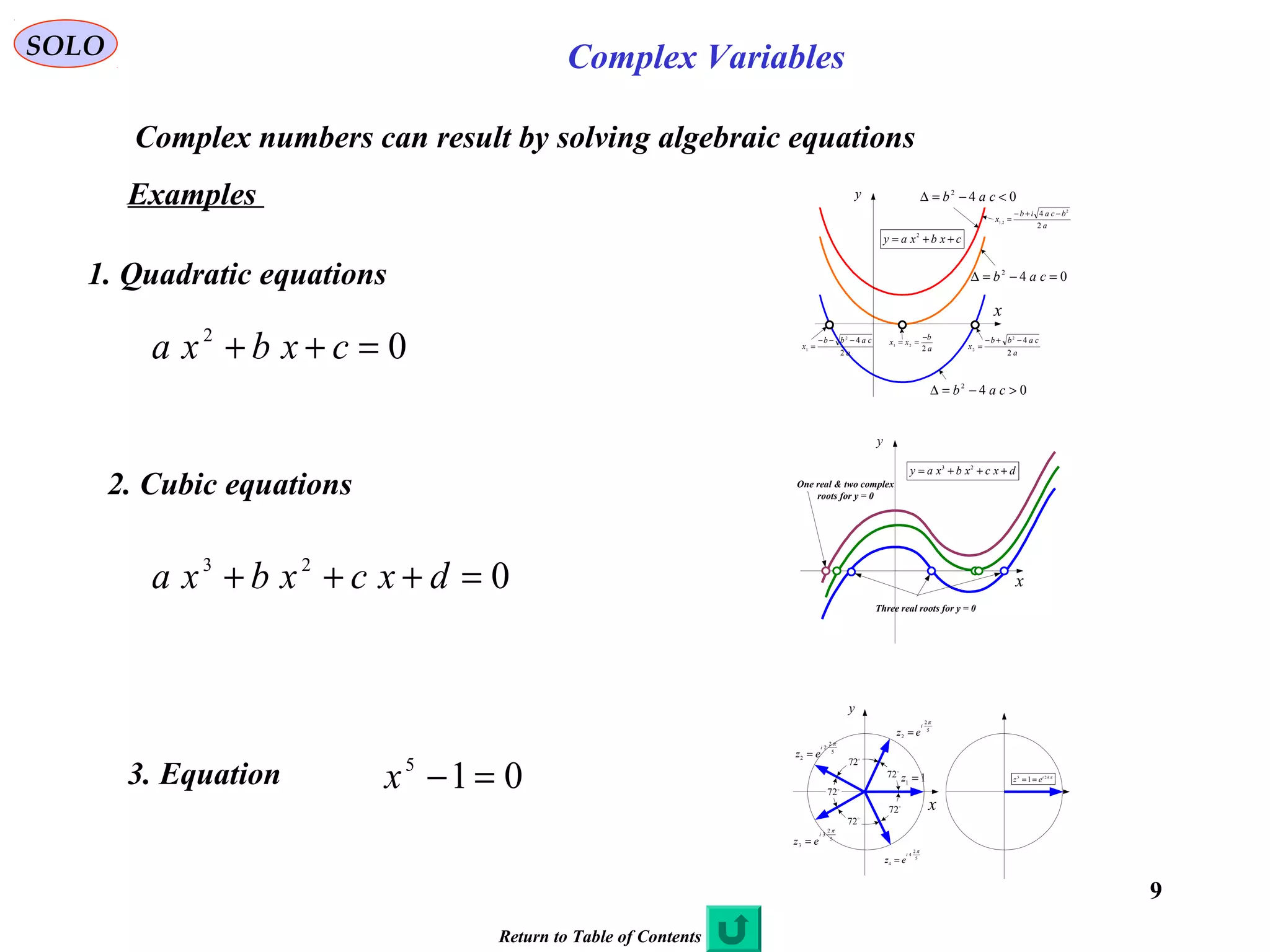
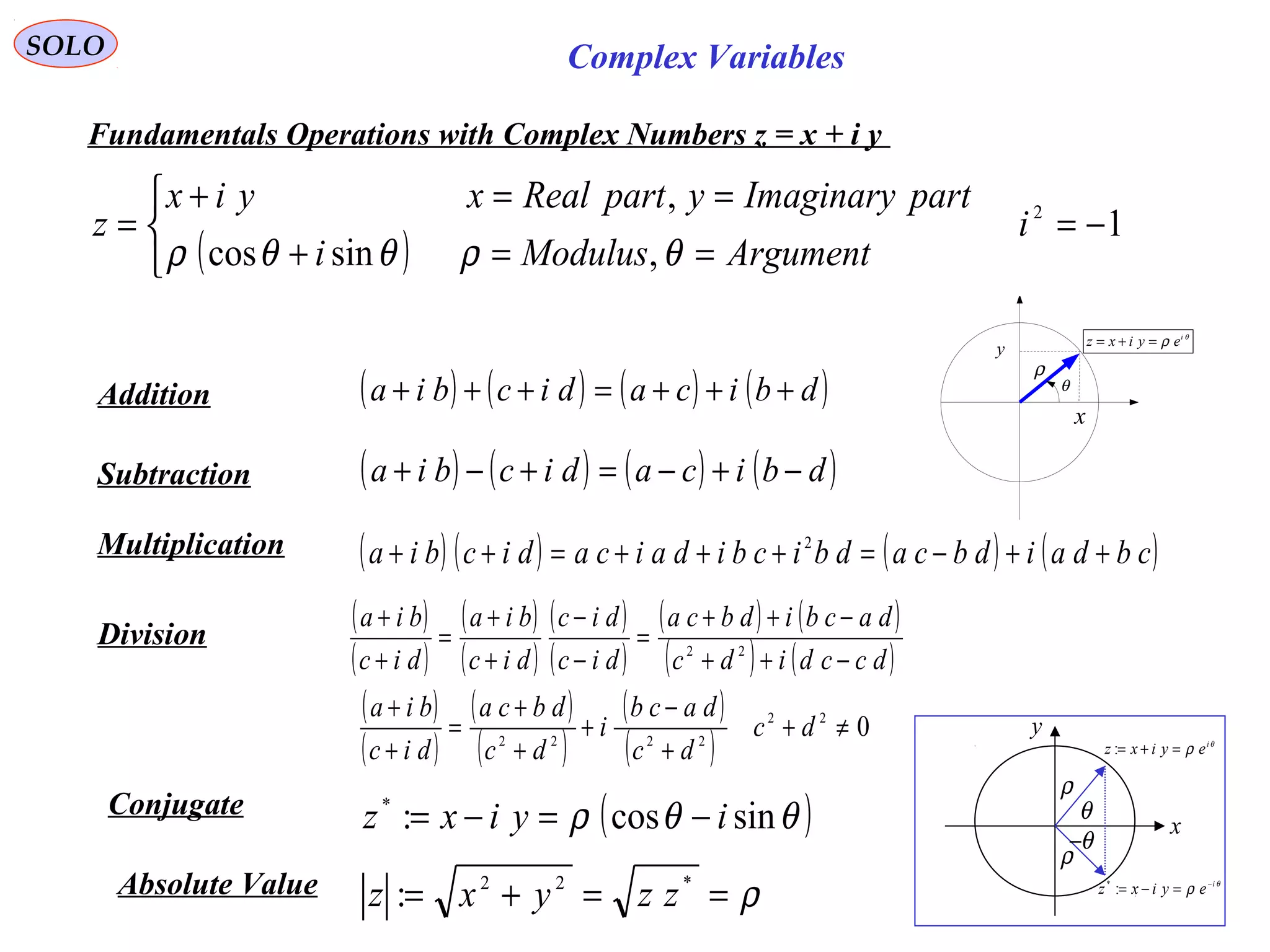
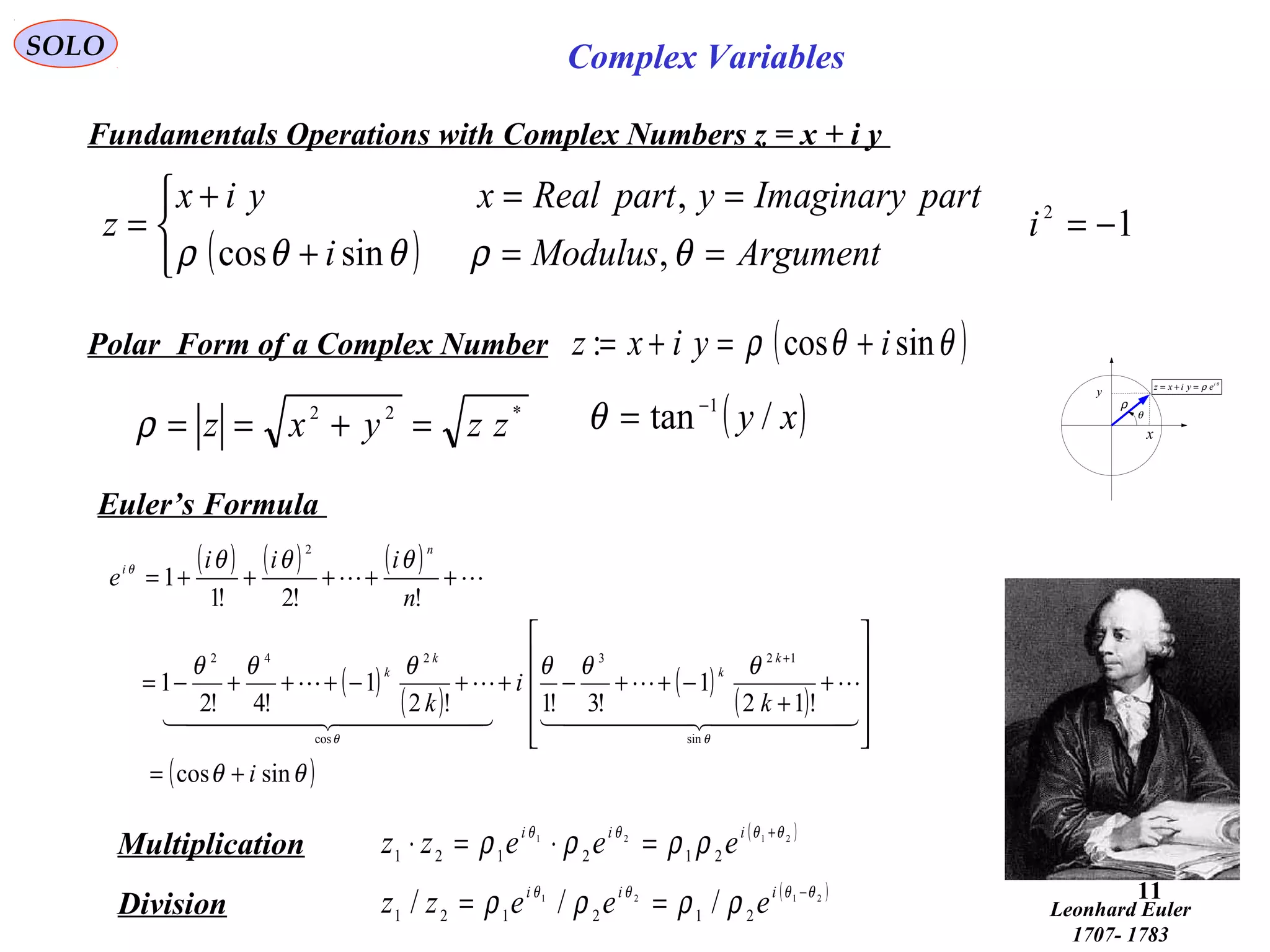
Fundamentals Operations with Complex Numbers z = x + i y
1
,
, 2
−=
==
==+
= i
ArgumentModuluse
partImaginaryypartRealxyix
z i
θρρ θ
θ
ρ i
eyixz =+=
y
x
ρ
θ
Polar Form of a Complex Number θ
ρ i
eyixz =+=:
De Moivre Theorem
( )[ ] ( )
( )θθρρ
ρθθρ
θ
θ
nine
eiz
nnin
ninn
sincos
sincos
+==
=+=
Roots of a Complex Number
[ ]
( ) ( )[ ]
1.2.1.0
2
sin
2
cos
sincos
/1
/1/12/1
−=
+
+
+
=
+== +
nk
n
k
i
n
k
iez
n
nnkin
πθπθ
ρ
θθρρ πθ
πki
ez 25
1==
y
x
5
2
2
π
i
ez =
5
2
2
2
π
i
ez =
5
2
3
3
π
i
ez =
5
2
4
4
π
i
ez =
11
=z
72
72
72
72
72
Abraham De Moivre
1667 - 1754
Return to Table of Contents](https://image.slidesharecdn.com/complexvariables-140921180830-phpapp02/75/Mathematics-and-History-of-Complex-Variables-12-2048.jpg)
![15
SOLO Complex Variables
History of Complex Numbers
Abraham bar Hiyya Ha-Nasi הנשיא חייא בר אברהם
writes the work Hibbur ha-Meshihah ve-ha-Tishboret
והתשבורת המשיחה חבור , translated in 1145 into Latin as Liber
embadorum, which presents the first complete solution to the
quadratic equation.
Abraham bar Hiyya Ha-Nasi (הנשיא חייא בר אברהם Abraham son of
[Rabbi] Hiyya "the Prince") (1070 - 1136?) was a Spaish Jewish
Mathematician and astronomer, also known as Savasorda (from the
Arabic الشرطة صاحب Sâhib ash-Shurta "Chief of the Guard"). He
lived in Barcelona.
Abraham bar iyya ha-NasiḤ [2]
(1070 – 1136 or 1145)](https://image.slidesharecdn.com/complexvariables-140921180830-phpapp02/75/Mathematics-and-History-of-Complex-Variables-15-2048.jpg)
![30
SOLO Complex Variables
Analytic, Holomorphic, MeromorphicFunctions
Return to Table of Contents
A Meromorphic Function on an open subset D of the complex plane is a
function that is Holomorphic on all D except a set of isolated points, which are
poles for the function. (The terminology comes from the Ancient Greek meros
(μέρος), meaning “part”, as opposed to holos ( λος)ὅ , meaning “whole”.)
The word “Holomorphic" was introduced by two of Cauchy's students, Briot
(1817–1882) and Bouquet (1819–1895), and derives from the Greek λοςὅ
(holos) meaning "entire", and μορφή (morphē) meaning "form" or
"appearance".[2]
Today, the term "holomorphic function" is sometimes preferred to "analytic
function", as the latter is a more general concept. This is also because an
important result in complex analysis is that every holomorphic function is
complex analytic, a fact that does not follow directly from the definitions. The
term "analytic" is however also in wide use.
The Gamma Function is Meromorphic in the
whole complex plane
Poles](https://image.slidesharecdn.com/complexvariables-140921180830-phpapp02/75/Mathematics-and-History-of-Complex-Variables-30-2048.jpg)
![34
SOLO Complex Variables
Singular Points
A point at which f (z) is not analytic is called a singular point. There are various types
of singular points:
3. Branch Points
If f (z) is a multiple valued function at z0, then this is a branch point.
Examples:
( ) ( ) n
zzzf
/1
0−= has a branch point at z=z0
( ) ( ) ( )[ ]0201ln zzzzzf −−= has a branch points at z=z01 and z=z02
4. Removable Singularities
The singular point z0 is a removable singularity of f (z) if exists.( )zf
zz 0
lim
→
Examples: The singular point z = 0 of is a removable singularity
z
zsin
1
sin
lim0
=→
z
z
z](https://image.slidesharecdn.com/complexvariables-140921180830-phpapp02/75/Mathematics-and-History-of-Complex-Variables-34-2048.jpg)
![37
SOLO Complex Variables
Complex Line Integrals
Let f (z) be continuous at all points on a curve C of a finite length L.
( ) ( ) ( )∑∑ ==
− ∆=−=
n
i
ii
n
i
iiin zfzzfS
11
1 ξξ
C
1
z
nzb =
2z
0
za =
1−iz
iz
1
ξ
2
ξ
i
ξ
n
ξ
Let subdivide C into n parts by n arbitrary points
z1, z2,…,zn, and call a=z0 and b=zn. On each arc joining
zi-1 to zi choose a point ξi. Define the sum:
Let the number of subdivisions n increase in such a
way that the largest of Δzi approaches zero, then the sum approaches a limit
that is called the line integral (also Riemann-Stieltjes integral).
( ) ( ) ( )∫∫∑ ==∆=
=
→∆∞→
C
b
a
n
i
ii
z
nn
zdzfzdzfzfS
i
1
0
limlim ξ
Properties of Integrals
( ) ( )[ ] ( ) ( )∫∫∫ +=+
CCC
zdzgzdzfzdzgzf ( ) ( ) constantAzdzfAzdzfA
CC
== ∫∫
( ) ( )∫∫ −=
a
b
b
a
zdzfzdzf ( ) ( ) ( )∫∫∫ +=
b
c
c
a
b
a
zdzfzdzfzdzf
( ) ( ) ( ) CoflengthLandConMzfLMzdzfzdzf
CC
≤≤≤ ∫∫
Return to Table of Contents](https://image.slidesharecdn.com/complexvariables-140921180830-phpapp02/75/Mathematics-and-History-of-Complex-Variables-37-2048.jpg)
![40
SOLO Complex Variables
Proof of Green’s Theorem in the Plane C
R
P
T
S
Q
a b
x
y
( )xgy 2=
( )xgy 1=
Start with a region R and the boundary curve C, defined
by S,Q,P,T, where QP and TS are parallel with y axis.
( )
( )
∫ ∫∫∫
=
=
∂
∂
=
∂
∂
b
a
xgy
Xgy
dy
y
P
dxdydx
y
P
2
R
By the fundamental lemma
of integral calculus:
( )
( )
( )
( ) ( )
( )
( )[ ] ( )[ ]xgxPxgxPyxPdy
y
yxP xgy
xgy
xgy
Xgy
12
,,,
, 2
1
2
−==
∂
∂ =
=
=
=
∫
Therefore: ( )[ ] ( )[ ]∫∫∫∫ −=
∂
∂
b
a
b
a
dxxgxPdxxgxPdydx
y
P
12
,,
R
but: ( )[ ] ( )[ ]∫∫ =
a
bSQ
dxxgxPdxxgxP 22
,, integral along curve SQ
( )[ ] ( )[ ]∫∫ =
b
aPT
dxxgxPdxxgxP 11
,, integral along curve PT
If we add to those integrals: ( ) ( ) 00,, === ∫∫ dxsincedxyxPdxyxP
QPTS
we
obtain:
( )[ ] ( ) ( )[ ] ( ) ( )∫∫∫∫∫∫∫ −=−−−−=
∂
∂
CTSPTQPSQ
dxyxPdxyxPdxxgxPdxyxPdxxgxPdydx
y
P
,,,,, 12
R
Assume that PT is defined by the function y = g1 (x) and
SQ is defined by the function y = g2 (x), both smooth and
y
P
∂
∂
is continuous in R:](https://image.slidesharecdn.com/complexvariables-140921180830-phpapp02/75/Mathematics-and-History-of-Complex-Variables-40-2048.jpg)
![47
SOLO Complex Variables
Proof of Cauchy-Goursat Theorem (continue – 2)
C
F
DE
A
B
I
∆
IV
∆
II
∆ III
∆
( ) ( )∫∫ ∆∆
≤
n
dzzfdzzf n
4
For an analytic function f (z) compute ( )
( ) ( )
( )0
0
0
0
':, zf
zz
zfzf
zz −
−
−
=η
( )
( ) ( )
( ) ( ) ( ) 0'''lim,lim 000
0
0
0
00
=−=
−
−
−
= →→
zfzfzf
zz
zfzf
zz zzzz
η
( ) ( ) ( ) ( ) ( ) ( ) ( )0000000
,'&,..,0 zzzzzzzfzfzfzzwheneverzzts −+−+=<−<∃>∀ ηδεηδε
( ) ( ) ( ) ( )[ ] ( ) ( ) ( ) ( )∫∫∫∫ ∆∆
←
∆∆
−≤−+−+≤
nnnn
dzzzzzdzzzzzdzzzzfzfdzzf
TheoremIntegralCauchy
0000
0
)00 ,,' ηη
n∆
0z
na
nb
nc
z 0
zz −
0
zzcbaP nnnn
−≥++=
( ) ( ) ( )
2
2
00
2
,
==≤−≤ ∫∫∫ ∆∆∆
nnn
P
PdzPdzzzzzdzzf
nnn
εεεη
But , where Pn the perimeter
of Δn and P the perimeter of Δ are related, by construction, by
( ) δεη <≤−< n
Pzzzz 00
&,
n
n PP 2/=
q.e.d.
( ) ( ) ( ) 0
4
44
0
2
2
=→=≤≤ ∫∫∫ ∆
→
∆∆
dzzfP
P
dzzfdzzf n
nn
n
ε
εε](https://image.slidesharecdn.com/complexvariables-140921180830-phpapp02/75/Mathematics-and-History-of-Complex-Variables-47-2048.jpg)
![48
SOLO Complex Variables
Proof of Cauchy-Goursat Theorem (continue – 3)
n
z1
z
2
z
1−i
z
i
z
1−n
z
n
∆1∆
2∆
3
∆
i
∆
C
O
q.e.d.
For the general case of a simple closed curve C
we take n points on C: z1, z2,…,zn and a point
O inside C. We obtain n triangles Δ1, Δ2,.., Δn,
for each of them we proved Cauchy-Goursat Theorem.
Let define the sum: ( ) ∑= − −
∆=
n
i zz
iin
ii
zzfS
1
1
:
we have: ( ) ( ) ( ) ( ) 0
1
1
=++= ∫∫∫∫
−
−∆
i
i
i
ii
z
O
O
z
z
z
dzzfdzzfdzzfdzzf
( ) ( ) ( ) ( ) ( )[ ] ( ) ( )[ ] ( )
n
i
i
i
i
i
i
i
ii
S
n
i
z
z
i
n
i
z
z
i
n
i
z
z
ii
n
i
z
z
n
i
dzzfdzzfzfdzzfzfzfdzzfdzzf ∑ ∫∑∫∑ ∫∑ ∫∑ ∫ ===== ∆ −−−−
+−=+−===
11111
1111
0
( ) ( ) ( )ε
ε
NnforSdzzfdzzfS n
CC
nn
><−→= ∫∫∞→
2
lim
( ) ( )[ ] ( ) ( )[ ] ( )
221
1
111
11
εε
=−≤−≤−≤→−= ∑∑∑ ∫∑∫ =
−
===
−−
n
i
ii
n
i
i
n
i
z
z
in
n
i
z
z
in
zz
L
dzfzfdzzfzfSdzzfzfS
i
i
i
i
( ) ( ) ( ) ( ) 0
22
=→>=+<+−≤ ∫∫∫ C
nn
CC
dzzfNnforSSdzzfdzzf εε
εε
Since we proved that , we can write:( ) 0=∫∆
dzzf
Return to Table of Contents](https://image.slidesharecdn.com/complexvariables-140921180830-phpapp02/75/Mathematics-and-History-of-Complex-Variables-48-2048.jpg)
![50
SOLO Complex Variables
Cauchy’s Integral Formulas
Augustin Louis Cauchy
)1789-1857(
If f (z) is analytic inside and on a simple closed curve C
and a is any point inside C then
( ) ( )
∫ −
=
C
dz
az
zf
i
af
π2
1
C
x
y
R
a
Γ
Proof:
Let chose a circle Γ with center at a
[ ]{ }πθε θ
2,0,: ∈+==Γ i
eazz
Since f (z)/ (z-a) is analytic in the region defined
between C and the circle Γ we can use:
( ) ( )
∫∫ Γ
−
=
−
zd
az
zf
zd
az
zf
C
( ) ( ) ( ) ( )afidafidei
e
eaf
zd
az
zf i
i
i
πθθε
ε
ε
ππ
θ
θ
θ
ε
21lim
2
0
2
0
0
===
+
=
− ∫∫∫ →
Γ
therefore:
( ) ( )
∫ −
=
C
dz
az
zf
i
af
π2
1
q.e.d.
Cauchy’s Integral Formulas and Related Theorems
Return to Table of Contents](https://image.slidesharecdn.com/complexvariables-140921180830-phpapp02/75/Mathematics-and-History-of-Complex-Variables-50-2048.jpg)
![52
SOLO Complex Variables
Morera’s Theorem (the converse of Cauchy’s theorem)
If f (z) is continuous in a simply-connected region R and if
around every simple closed curve C in R then
f (z) ia analytic in R.
( ) 0=∫C
dzzf
B
x
y
R
A
C1
C2
D1
D2
a
z
Proof:
Since around every closed curve C in R( ) 0=∫C
dzzf
( ) ( ) ( ) ( ) ( ) ( ) ( )∫∫∫∫∫∫∫ =→−=+==
BDAcBDAcBDAcBDAcACBDBDAcACBDDAC
dzzfdzzfdzzfdzzfdzzfdzzfdzzf
2211221122111122
0
The integral is independent on path
between two points, if the path is in R
( ) ( )∫=
z
a
dzzfzF
Let choose a straight path between z and z+Δz
( ) ( ) ( ) ( ) ( ) ( ) ( ) ( )[ ]∫∫∫
∆+∆+
−
∆
=−
−
∆
=−
∆
−∆+
zz
z
z
a
zz
a
udzfuf
z
zfudufuduf
z
zf
z
zFzzF 11
Since f (z) is continuous ( ) ( ) δε <−≤− zuwheneverzfuf
Therefore
( ) ( ) ( ) ( ) ( ) ( ) ( )zf
zd
zFd
zudzfuf
z
zf
z
zFzzF
zz
z
=→<∆∀=−
∆
≤−
∆
−∆+
∫
∆+
δε
1
C
x
y
R z
Νδz+∆ z
Since F (z) has a derivative in R, it is analytic, and so are its derivatives, i.e. f (z)
Return to Table of Contents
Giacinto Morera
1856 - 1907](https://image.slidesharecdn.com/complexvariables-140921180830-phpapp02/75/Mathematics-and-History-of-Complex-Variables-52-2048.jpg)
![62
SOLO Complex Variables
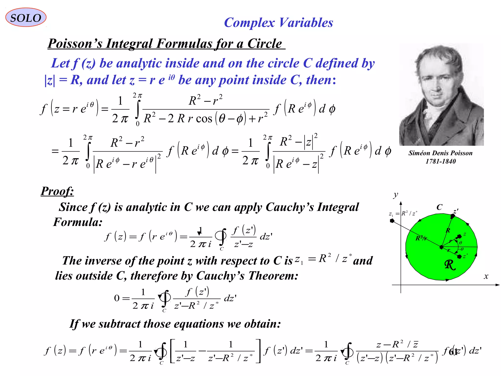
Poisson’s Integral Formulas for a Circle
Siméon Denis Poisson
1781-1840
Proof (continue):
( ) ( ) ( ) ( ) ( )
( )
( ) ( )[ ] ( )
( ) ( )
( )( ) ( )
( )
( )( ) ( )
( )
( )
( )∫
∫
∫
∫
∫
+−−
−
=
−−
−
=
−−
−
=
−−
−
=
−−
−
==
−−
+
∗
π
φ
π
φ
θφθφ
π
φ
θφθφ
φθ
π
φφ
θφθφ
θθ
θ
φ
φθπ
φ
π
φ
π
φ
π
π
2
0
22
22
2
0
22
2
0
22
2
0
2
2
2
2
cos22
1
2
1
2
1
/
/
2
1
''
/''
/
2
1
deRf
RrRr
rR
deRf
ereRereR
rR
deRf
eRerereR
eRr
deRieRf
erReRereR
erRer
i
dzzf
zRzzz
zRz
i
erfzf
i
i
iiii
i
iiii
i
ii
iiii
ii
C
i
Writing we have:( ) ( ) ( )θθθ
,, rviruerf i
+=
( ) ( )
( )
( )∫ +−−
−
=
π
φφ
φθπ
θ
2
0
22
22
,
cos22
1
, dRu
RrRr
rR
ru
( ) ( )
( )
( )∫ +−−
−
=
π
φφ
φθπ
θ
2
0
22
22
,
cos22
1
, dRv
RrRr
rR
rv
q.e.d.
C
x
y
R
R
z'
rR2/r
θ
∗
z
z
r θ−
∗
= zRz /2
1
Return to Table of Contents](https://image.slidesharecdn.com/complexvariables-140921180830-phpapp02/75/Mathematics-and-History-of-Complex-Variables-62-2048.jpg)
![81
SOLO Complex Variables
Weierstrass M (Majorant) Test
Karl Theodor Wilhelm
Weierstrass
(1815 – 11897)
The most commonly encountered test for Uniform
Convergence is the Weierstrass M Test.
Proof:
Since converges, some number N exists such that for n + 1 ≥ N,
If we can construct a series of numbers , in
which Mi ≥ |ui(x)| for all x in the interval [a,b] and
is convergent, the series ui(x) will be uniformly
convergent in [a,b].
∑
∞
1 iM
∑
∞
1 iM
∑
∞
1 iM
ε<∑
∞
+= 1ni
iM
This follows from our definition of convergence. Then, with |ui(x)| ≤ Mi for
all x in the interval a ≤ x ≤ b, ( ) ε<∑
∞
+= 1ni
i xu
Hence ( ) ( ) ( ) ε<=− ∑
∞
+= 1ni
in xuxsxS
and by definition is uniformly convergent in [a,b]. Since we
specified absolute values in the statement of the Weierstrass M Test, the
series is also Absolutely Convergent. Return to the Table of Content
∑
∞
=1i iu
∑
∞
=1i iu](https://image.slidesharecdn.com/complexvariables-140921180830-phpapp02/75/Mathematics-and-History-of-Complex-Variables-81-2048.jpg)
![SOLO Complex Variables
Abel’s Test
Niels Henrik Abel
( 1802 – 1829)
If
and the functions fn(x) are monotonic decreasing |
fn+1(x) ≤ fn(x)| and bounded, 0 ≤ fn(x) ≤ M, for all x in
[a,b], then Converges Uniformly in [a,b].
( ) ( )
convergentAa
xfaxu
n
nnn
,=
=
∑
( )∑n n xu
( ) ( ) [ ] ( ) [ ]bainconvergentuniformlyisxu
xd
d
baincontinuousarexu
xd
d
andxu n nnn ,&, 1∑
∞
=
Return to the Table of Content
Uniformly convergent series have three particular useful properties:
1.If the individual terms un(x) are continuous, the series sum
is also continuous.
2. If the individual terms un(x) are continuous, the series may be integrated term by term.
The sum of the integrals is equal to to the integral of the sum, then
3.The derivative of the series sum f (x) equals the sum of the individual term derivatives
providing the following conditions are satisfied
( ) ( )∑
∞
=
= 1n n xuxf
( ) ( )∑ ∫∫
∞
=
= 1n
b
a
n
b
a
xdxuxdxf
( ) ( )∑
∞
=
= 1n n xu
xd
d
xf
xd
d](https://image.slidesharecdn.com/complexvariables-140921180830-phpapp02/75/Mathematics-and-History-of-Complex-Variables-82-2048.jpg)
![109
SOLO Complex Variables
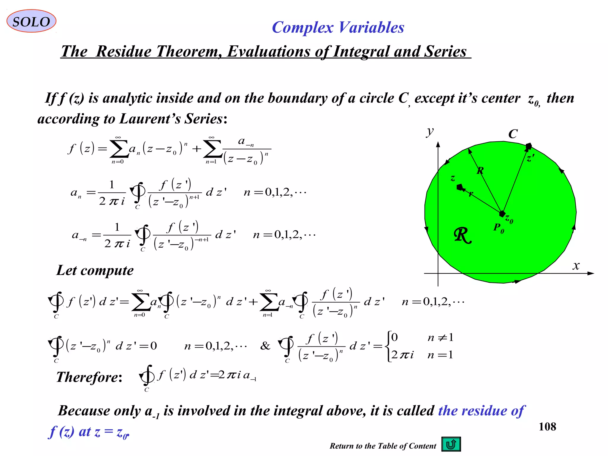
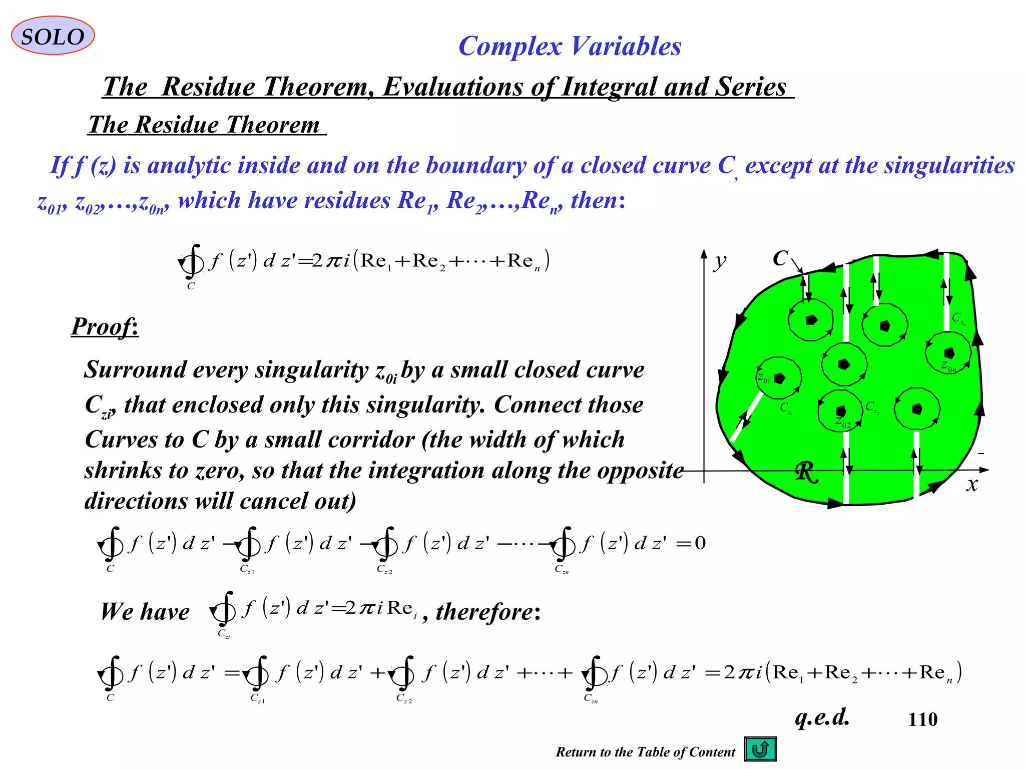
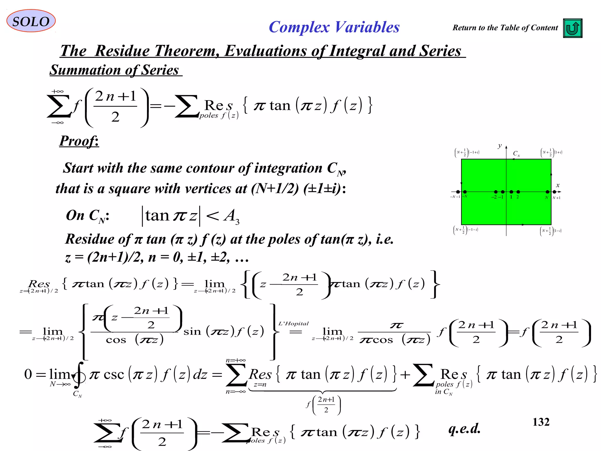
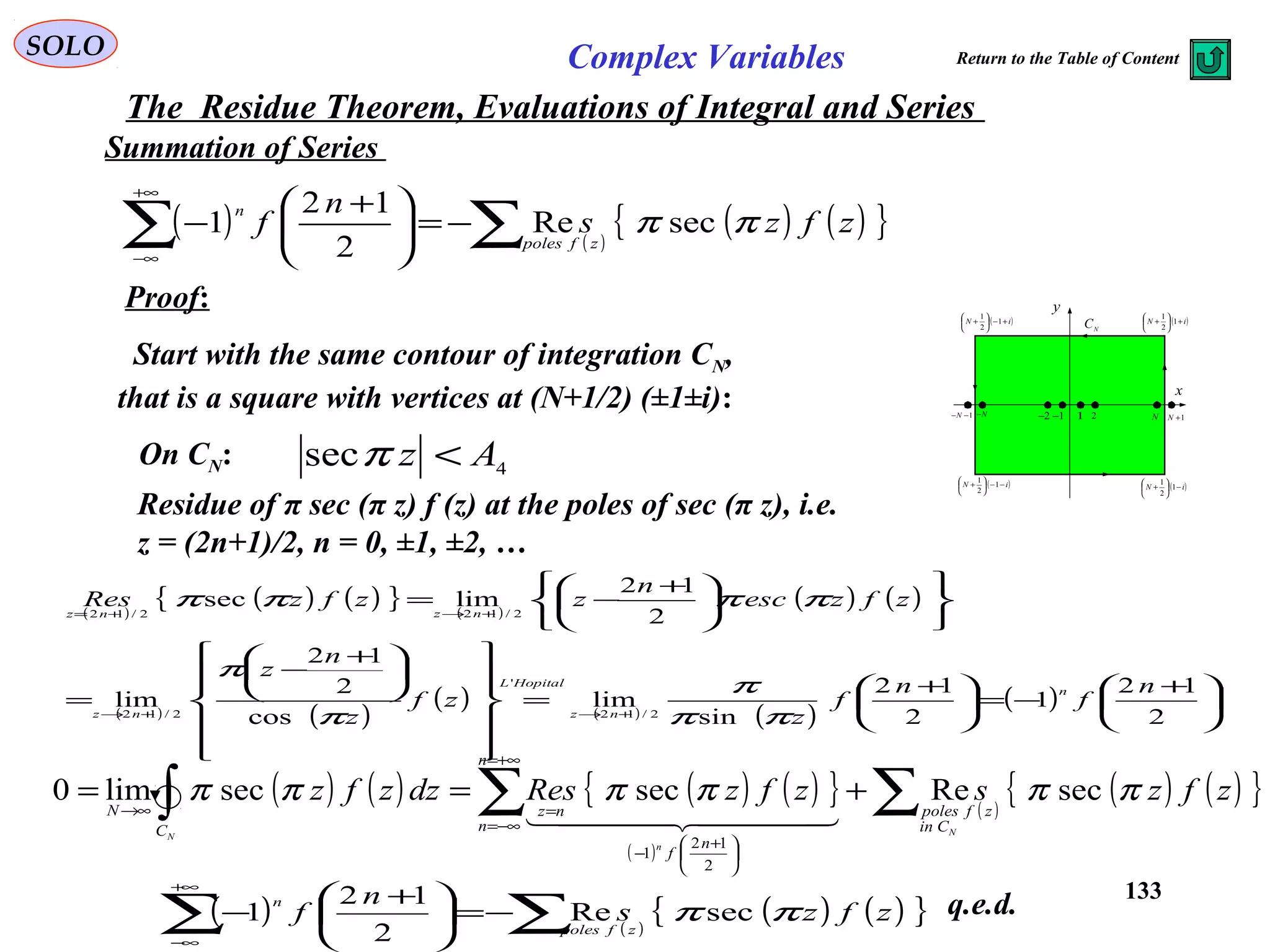
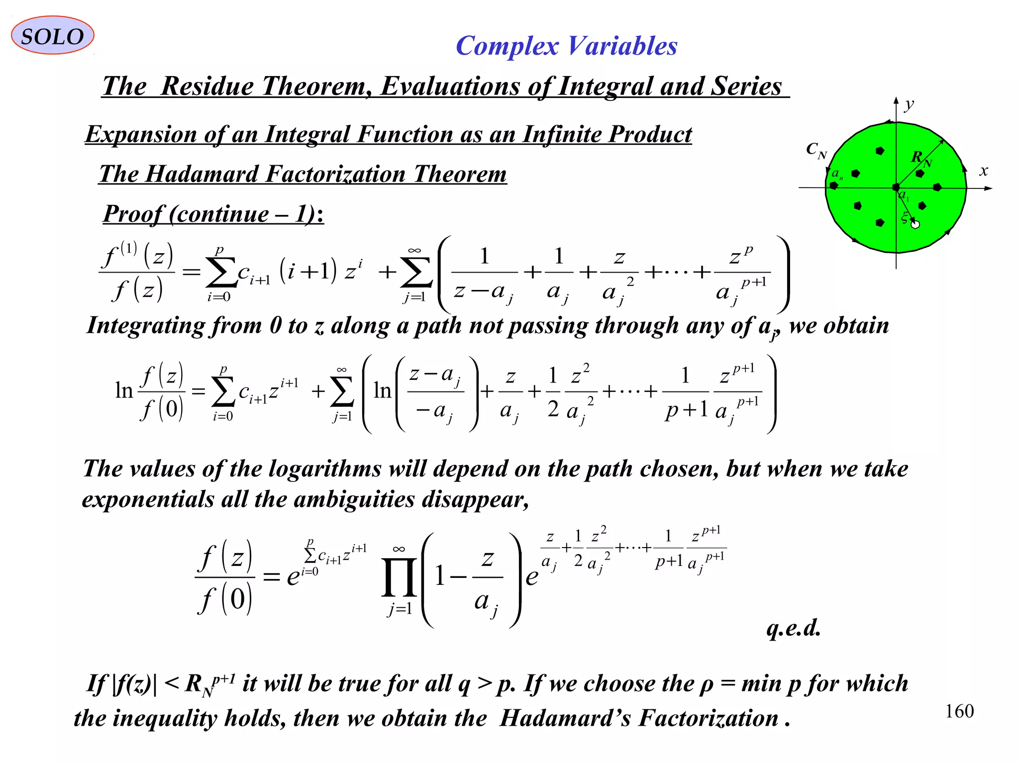
The Residue Theorem, Evaluations of Integral and Series
According to residue definition the residue of f (z) at z = z0 can be computed as follows:
C
x
y
R
R
z0
z
z'
r
P0
If z = z0 is a pole of order k, i.e. the Laurent series at
z0 is
Then:
( )∫=−
C
zdzf
i
a ''
2
1
1
π
Calculation of the Residues
( ) ( ) ( )
( ) ( ) +−+−++
−
++
−
+
−
= −−− 2
02010
0
2
0
2
0
1
zzazzaa
zz
a
zz
a
zz
a
k
k
( )
( ) ( )[ ]zfzz
zd
d
k
a
k
k
k
zz 01
1
1
!1
1
lim
0
−
−
= −
−
→−
( ) ( ) ( ) ( ) ( ) ( ) ( ) +−+−+−+++−+−=−
++
−
−
−
−
−
2
02
1
0100
2
02
1
010
kkk
k
kkk
zzazzazzaazzazzazfzz
and:
If z = z0 is a pole of order k=1, then:
( ) ( )[ ]zfzza
zz 01
0
lim −=
→−
( ) ( )
( )∑∑ =
−
∞
= −
+−=
k
n
n
n
n
n
n
zz
a
zzazf
1 00
0
Return to the Table of Content](https://image.slidesharecdn.com/complexvariables-140921180830-phpapp02/75/Mathematics-and-History-of-Complex-Variables-109-2048.jpg)

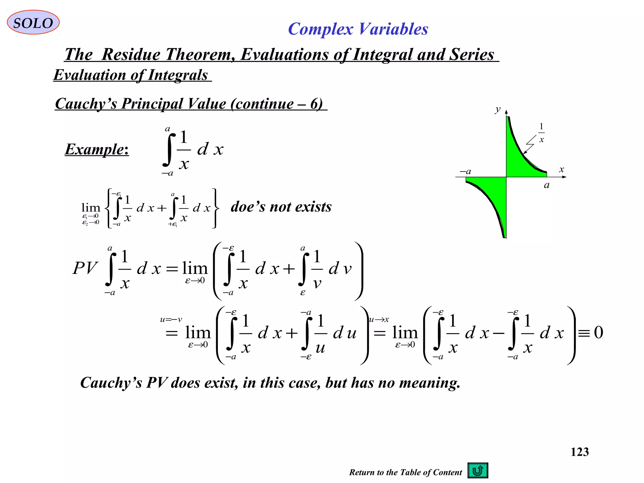
![119
SOLO Complex Variables
The Residue Theorem, Evaluations of Integral and Series
Evaluation of Integrals
Cauchy’s Principal Value (continue – 2)
Theorem 2:
If F (z) is analytic on and inside a positive-sensed circle C of radius ε, except at the
center of C, z = z0, that is a simple pole of F (z), then
C
x
y ψC
0
z
0
θ
0
θψ +
ψ
ε
O
( ) ( )[ ]0
0
lim zFResizdzF
C
ψ
ψ
ε
=∫→
where Cψ is every arc on C of angle ψ.
Proof:
Since f (z) is analytic inside and on C by using Theorem 1 we obtain the
desired result.
The function:
( )
( ) ( )
( )[ ] ( ) ( )[ ]
=−=
≠−
=
→
000
00
0
lim zzzFzzzFRes
zzzFzz
zf
zz](https://image.slidesharecdn.com/complexvariables-140921180830-phpapp02/75/Mathematics-and-History-of-Complex-Variables-119-2048.jpg)
![120
SOLO Complex Variables
The Residue Theorem, Evaluations of Integral and Series
Evaluation of Integrals
Cauchy’s Principal Value (continue – 3)
Theorem 3:
If F (z) is analytic on and inside a positive-sensed curve C, except at the interior poles
zint1, zint2,…, zint n and the simple poles on the curve C, zcont1, zcont2,…, zcont m,
then
Proof:
x
y
1intz
2intz
n
zint
1+scontext
z
2cz
ck
z
1c
ε
2c
ε
0
C
2+scontext
z
1in tcont
z
2intcontz
mcontext
z
scontz int
scontint
ε
mcontext
ε
2intcont
ε
2+scontext
ε
1+scontext
ε
2in tcontCz
2+scontext
Cz
1+scontext
Cz
1in tcont
Cz
mcontext
Cz
scont
Cz in t
∑=
+=
m
k
kcontCCC
1
0
( ) ( ) ( ) ( )[ ] ( )[ ]
+=++ ∑∑∑ ∫∑ ∫∫ ==+==
s
k
kcont
n
j
j
m
sk C
s
k CC
zFReszFResizdzFzdzFzdzF
kextcontkcont
1
int
1
int
11
2
int0
π
( ) ( )[ ] ( )[ ]
+= ∑∑∫ ==
m
k
kcont
n
j
j
C
zFReszFResizdzF
11
int
2
1
2π
Let encircle the simple poles zcont k on the C contour by
semicircles Ccont k of radiuses ε cont k such that,
randomly, zcont int 1,…, zcont int s, are inside the
integration contour, and zcont ext s+1,…,zcont ext m are
outside the integration contour. We have:
where](https://image.slidesharecdn.com/complexvariables-140921180830-phpapp02/75/Mathematics-and-History-of-Complex-Variables-120-2048.jpg)
![121
SOLO Complex Variables
The Residue Theorem, Evaluations of Integral and Series
Evaluation of Integrals
Cauchy’s Principal Value (continue – 4)
Proof (continue – 1):
x
y
1intz
2intz
n
zint
1+scontext
z
2cz
ck
z
1c
ε
2cε
0
C
2+scontext
z
1intcont
z
2intcontz
mcontext
z
scontz int
scontin t
ε
mcontext
ε
2in tcont
ε
2+scontext
ε
1+scontext
ε
2intcontCz
2+scontext
Cz
1+scontext
Cz
1intcont
Cz
mcontext
Cz
scont
Cz int
( ) ( )[ ]
= ∑∑ ∫ ==
→
s
k
kcont
s
k C
zFResizdzF
kcont
kcont
1
int
1
0
int
int
lim πε
The integrals along the semicircles Ccont k of the
singularities zcont ext s+1,…,zcont ext m that are
outside the integration contour, are in the negative
direction, and we have, according to Theorem 2:
( ) ( ) ( )[ ] ( )[ ]
+== ∑∑∫∫ ==
→
∑
m
k
kcont
n
j
j
CC
zFReszFResizdzFzdzF
c
11
int
0 2
1
2lim
0
π
ε
therefore:
Since the integrals along the semicircles Ccont k of the
singularities zcont int 1,…, zcont int s, that are inside the
integration contour, are in the positive direction we have,
according to Theorem 2:
( ) ( )[ ]
−= ∑∑ ∫ +=+=
→
m
sk
kextcont
m
sk C
zFResizdzF
kextcont
kcont
11
0int
lim πε
( ) ( ) ( ) ( )[ ] ( )[ ]
+=++ ∑∑∑ ∫∑ ∫∫ ==+==
s
k
kcont
n
j
j
m
sk C
s
k CC
zFReszFResizdzFzdzFzdzF
kextcontkcont
1
int
1
int
11
2
int0
π
Note: This result is independent on the way that we encircled the simple poles on
the curve C.
q.e.d.](https://image.slidesharecdn.com/complexvariables-140921180830-phpapp02/75/Mathematics-and-History-of-Complex-Variables-121-2048.jpg)
![125
SOLO
Example 2
0,
1
21
2
1
>∫−
RRxd
x
R
R
kLet compute: for k integer and positive
x
y
R
ε
A
B
C
D
E
F
G
H
Rx =Rx −=
This integral has a singularity on the path of
integration on x = 0:
Complex Variables
( )
( ) ( )[ ]
>
≤<
=+−−+−−=
−−=
+=
−−−−
→
→
−
−
−
−
→
→
−
−→
→
−
∫∫∫
1
100
lim
lim
11
lim
1
1
2
1
2
1
1
1
1
0
0
11
0
0
0
0
2
1
2
2
1
1
2
1
2
2
1
12
1
2
1
kdefinednot
k
kRkRkk
xkxkxd
x
xd
x
xd
x
kkkk
R
k
R
k
R
k
R
k
R
R
k
εε
ε
ε
ε
ε
ε
ε
ε
ε
ε
ε
Let compute:
( )
( ) ( ) ( )
( )
>
≤<
=
−
−
−+−−+−−=
−+−=
++=
−
−
−−−−
→
−
−
−
−
→
−
−
→
−
∫∫∫∫∫
oddk
k
e
k
kRkRkk
xk
eR
deRi
xkxd
x
zd
z
xd
x
xd
x
ki
k
kkkk
R
k
kik
i
R
k
R
k
C
k
R
k
R
R
k
&10
100
1
1
lim
lim
111
lim
1
2
1
11
2
1
1
1
0
1
0
1
00
2
2
1
1
2
1
2
1
π
ε
ε
π
θ
θ
ε
ε
εε
ε
ε
ε
εε
θ](https://image.slidesharecdn.com/complexvariables-140921180830-phpapp02/75/Mathematics-and-History-of-Complex-Variables-125-2048.jpg)
![170
SOLO Complex Variables
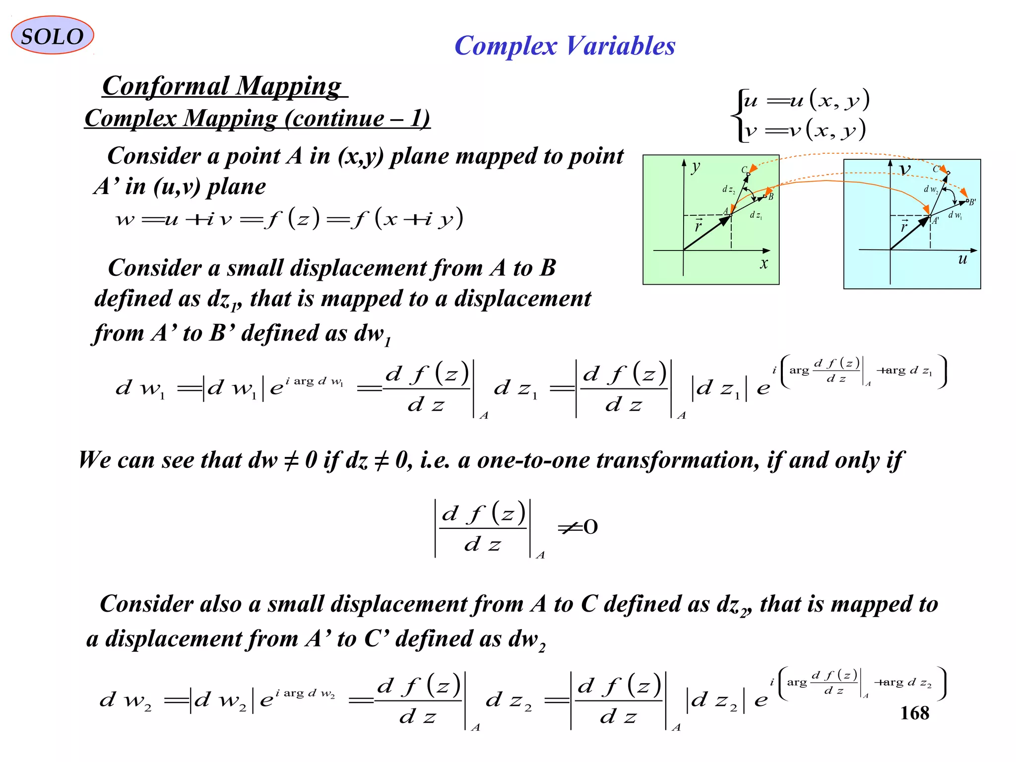
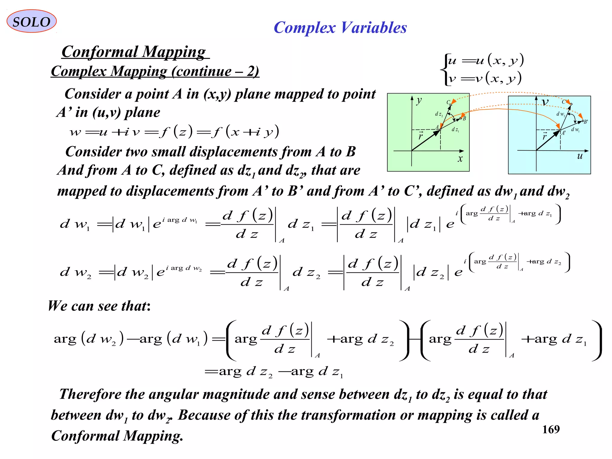
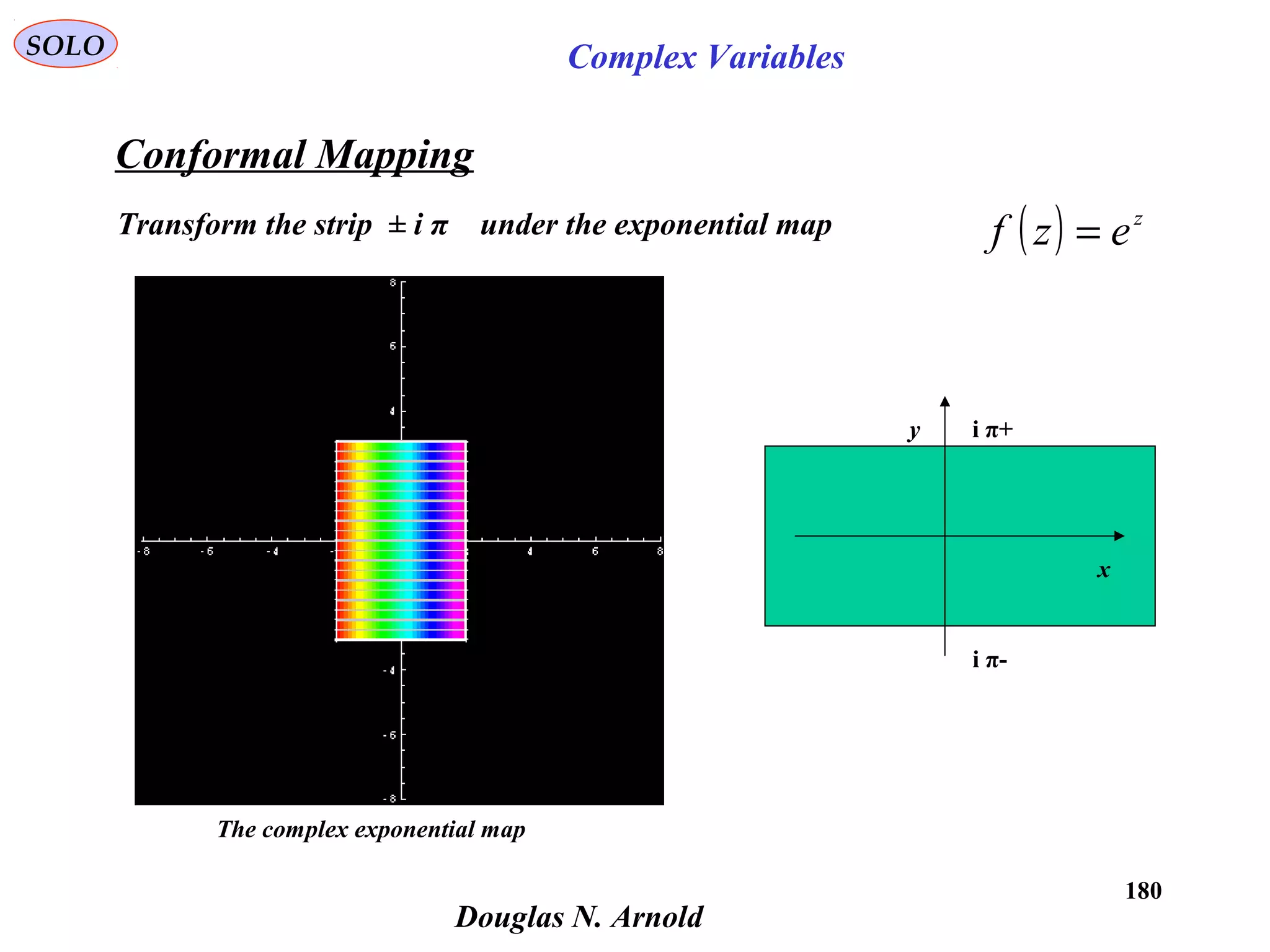
Conformal Mapping
( ) ( )[ ] RzRzzzf ≤−±=
2/122
ln
( )
( )
( ) ( )( ) z
Rzz
RzzR
Rzz
Rzz
R
Rzz
w
R
w 2222
2/1222
2/122
2/122
2
2/122
2
=
+−
−
+−±=
−±
+−±=+
Define ( ) ( ) RzRzzzgw ≤−±==
2/122
+=
w
R
w
2
1
z
2
( ) ( )
( ) ( )
( ) ( ) ( ) ( )
−++=
+
++=+
w
w
R
w
w
R
wwiww
2
1
wwiww
R
wwiww
2
1
yix
argsinargcosargsinargcos
argsinargcos
argsinargcos
22
2
( ) ( )
−=
+=
w
R
ww
2
1
y
w
R
ww
2
1
x
22
argsin&argcos](https://image.slidesharecdn.com/complexvariables-140921180830-phpapp02/75/Mathematics-and-History-of-Complex-Variables-170-2048.jpg)
![171
SOLO Complex Variables
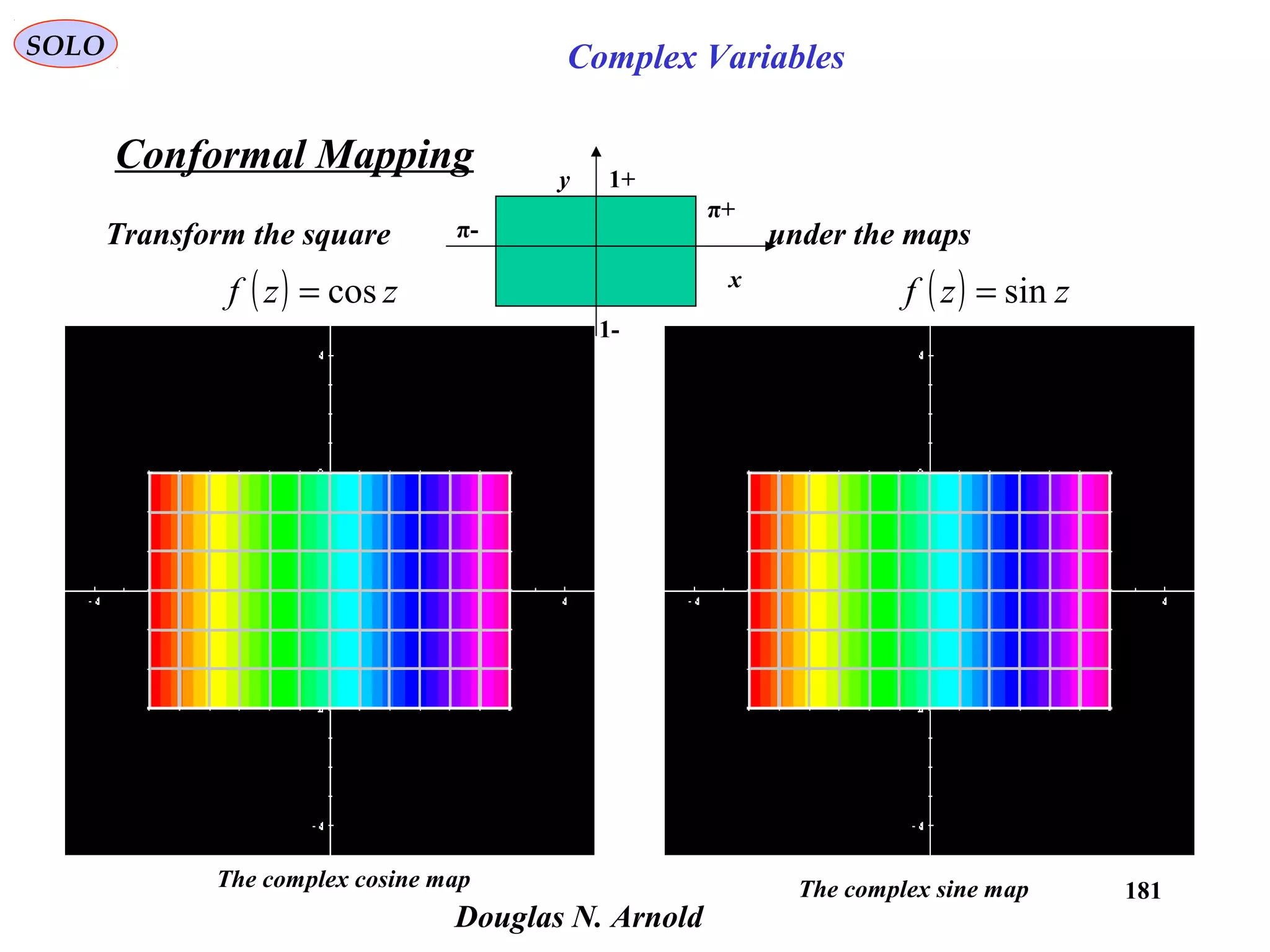
Conformal Mapping
( ) ( )[ ] RzRzzzf ≤−±=
2/122
ln
Define ( ) ( ) RzRzzzgw ≤−±==
2/122
( ) ( )
−=
+=
w
R
ww
2
1
y
w
R
ww
2
1
x
22
argsin&argcos
From those equations we have:
( ) ( )
2
2
2
2
2
22
4
1
4
1
argsinargcos
R
w
R
w
w
R
w
w
y
w
x
=
−−
+=
−
4
1
w
R
w
y
w
R
w
x
=
−
+
+
2
2
2
2
x
y
( )warg
wln
( ) ( )wiwzf argln +=](https://image.slidesharecdn.com/complexvariables-140921180830-phpapp02/75/Mathematics-and-History-of-Complex-Variables-171-2048.jpg)
![172
SOLO Complex Variables
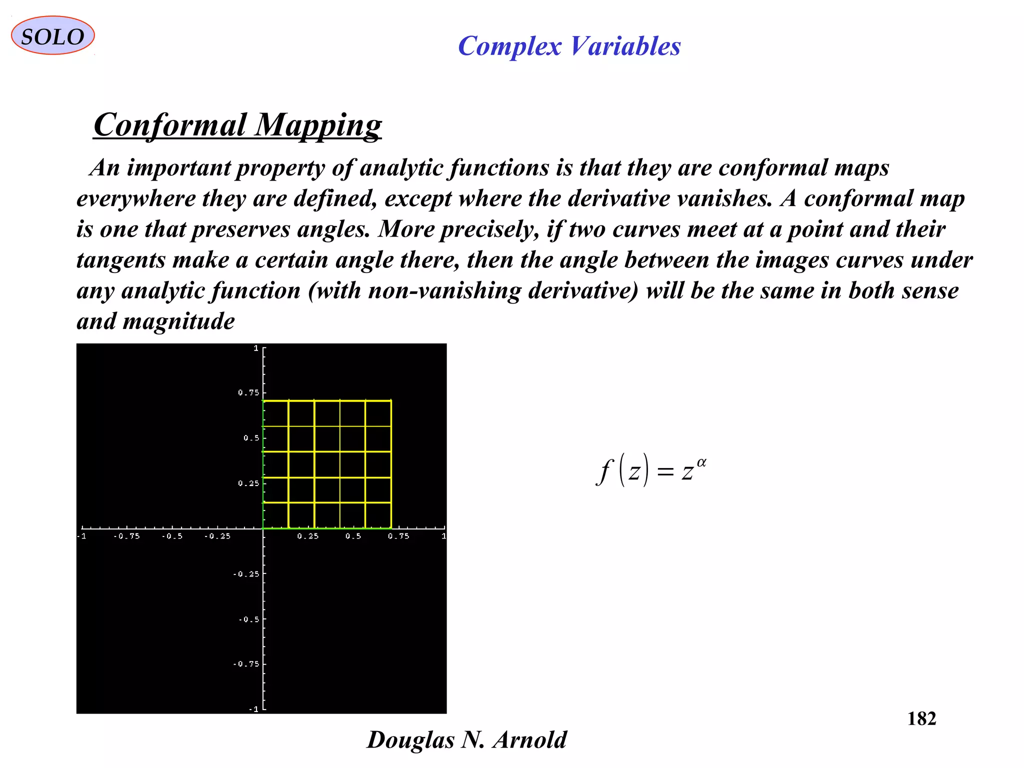
Conformal Mapping
( ) 2/tt
eex −
+=
0122
=+− tt
exe
( ) ( ) 2/cosh tt
eet −
+=
( ) ( )[ ]2/12
1ln −±= xxxacosh
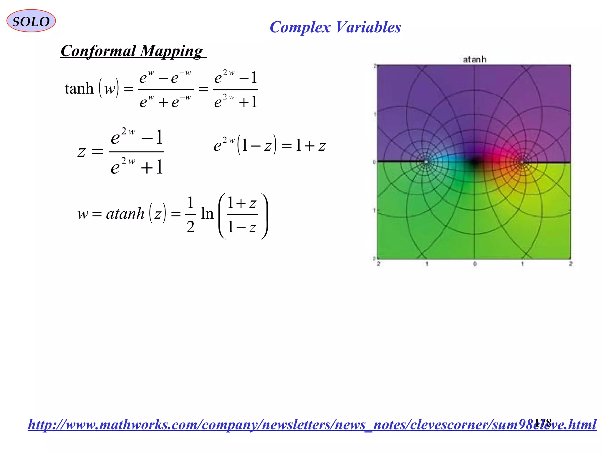
http://www.mathworks.com/company/newsletters/news_notes/clevescorner/sum98cleve.html](https://image.slidesharecdn.com/complexvariables-140921180830-phpapp02/75/Mathematics-and-History-of-Complex-Variables-172-2048.jpg)
![173
SOLO Complex Variables
Conformal Mapping
( ) ( )[ ]2/122
ln Rzzzf +±=
( )
( )
( ) ( )( ) z
Rzz
RzzR
Rzz
Rzz
R
Rzz
w
R
w 2222
2/1222
2/122
2/122
2
2/122
2
=
−−
+
−+±=
+±
−−±=−
Define ( ) ( ) 2/122
Rzzzgw +±==
−=
w
R
w
2
1
z
2
( ) ( )
( ) ( )
( ) ( ) ( ) ( )
+−+=
+
−+=+
w
w
R
w
w
R
wwiww
2
1
wwiww
R
wwiww
2
1
yix
argsinargcosargsinargcos
argsinargcos
argsinargcos
22
2
( ) ( )
+=
−=
w
R
ww
2
1
y
w
R
ww
2
1
x
22
argsin&argcos](https://image.slidesharecdn.com/complexvariables-140921180830-phpapp02/75/Mathematics-and-History-of-Complex-Variables-173-2048.jpg)
![174
SOLO Complex Variables
Conformal Mapping
( ) ( )[ ]2/122
ln Rzzzf +±=
Define ( ) ( ) 2/122
Rzzzgw +±==
( ) ( )
+=
−=
w
R
ww
2
1
y
w
R
ww
2
1
x
22
argsin&argcos
From those equations we have:
( ) ( )
2
2
2
2
2
22
4
1
4
1
argsinargcos
R
w
R
w
w
R
w
w
y
w
x
−=
+−
−=
−
4
1
w
R
w
y
w
R
w
x
=
+
+
−
2
2
2
2
x
y( )warg
wln
( ) ( )wiwzf argln +=](https://image.slidesharecdn.com/complexvariables-140921180830-phpapp02/75/Mathematics-and-History-of-Complex-Variables-174-2048.jpg)
![175
SOLO Complex Variables
Conformal Mapping
http://www.mathworks.com/company/newsletters/news_notes/clevescorner/sum98cleve.html
( ) 2/tt
eex −
−=
0122
=−− tt
exe
( ) ( ) 2/sinh tt
eet −
−=
( ) ( ) ( )[ ]2/12
1ln +±== zzzasinh:zf](https://image.slidesharecdn.com/complexvariables-140921180830-phpapp02/75/Mathematics-and-History-of-Complex-Variables-175-2048.jpg)
![176
SOLO Complex Variables
Conformal Mapping
dz
dz
kviuw
+
−
=+= ln
( )
( )
ku
e
ydx
ydx
dz
dz /2
22
222
=
++
+−
=
+
−
( ) ( )
( ) ( ) dx
dyx
ydxydx
ydxydx
e
e
k
u
ku
ku
21
1
coth
222
2222
2222
/2
/2
−
++
=
−+−+−
++++−
=
−
+
=
( )[ ] ( )[ ] ( )kudkudykudx /sinh/1/coth/coth 222222
=−=++
kvikukviku
ee
dz
dz
ee
dz
dz //// −
∗
∗
=
+
−
→=
+
−
dyi
dyx
i
dzdz
dzz
i
dz
dz
dz
dz
dz
dz
dz
dz
i
ee
ee
i
k
u
ctg kvikvi
kvikvi
2
2222
//
//
−+
=
−
−
=
+
−
−
+
−
+
−
+
+
−
=
−
+
=
∗
∗
∗
∗
∗
∗
−
−
( )[ ] ( )[ ] ( )kvdkvctgdkvctgdyx /sin/1// 222222
=+=++
kviku
ee
dz
dz //
=
+
−](https://image.slidesharecdn.com/complexvariables-140921180830-phpapp02/75/Mathematics-and-History-of-Complex-Variables-176-2048.jpg)
![177
SOLO Complex Variables
Conformal Mapping
dz
dz
kviuw
+
−
=+= ln
( )[ ] ( )kudykudx /sinh//coth 2222
=++
( )[ ] ( )kvdkvctgdyx /sin// 2222
=++
dd−
x
y
( )[ ] ( )kvdkvctgdyx /sin// 2222
=++
( )[ ] ( )kudykudx /sinh//coth 2222
=++
1v
2
v
3v
3
u
2u
1
u
We have two families of orthogonal circles.
All those circle passe through (-d,0) and (d,0)
v
u](https://image.slidesharecdn.com/complexvariables-140921180830-phpapp02/75/Mathematics-and-History-of-Complex-Variables-177-2048.jpg)
![190
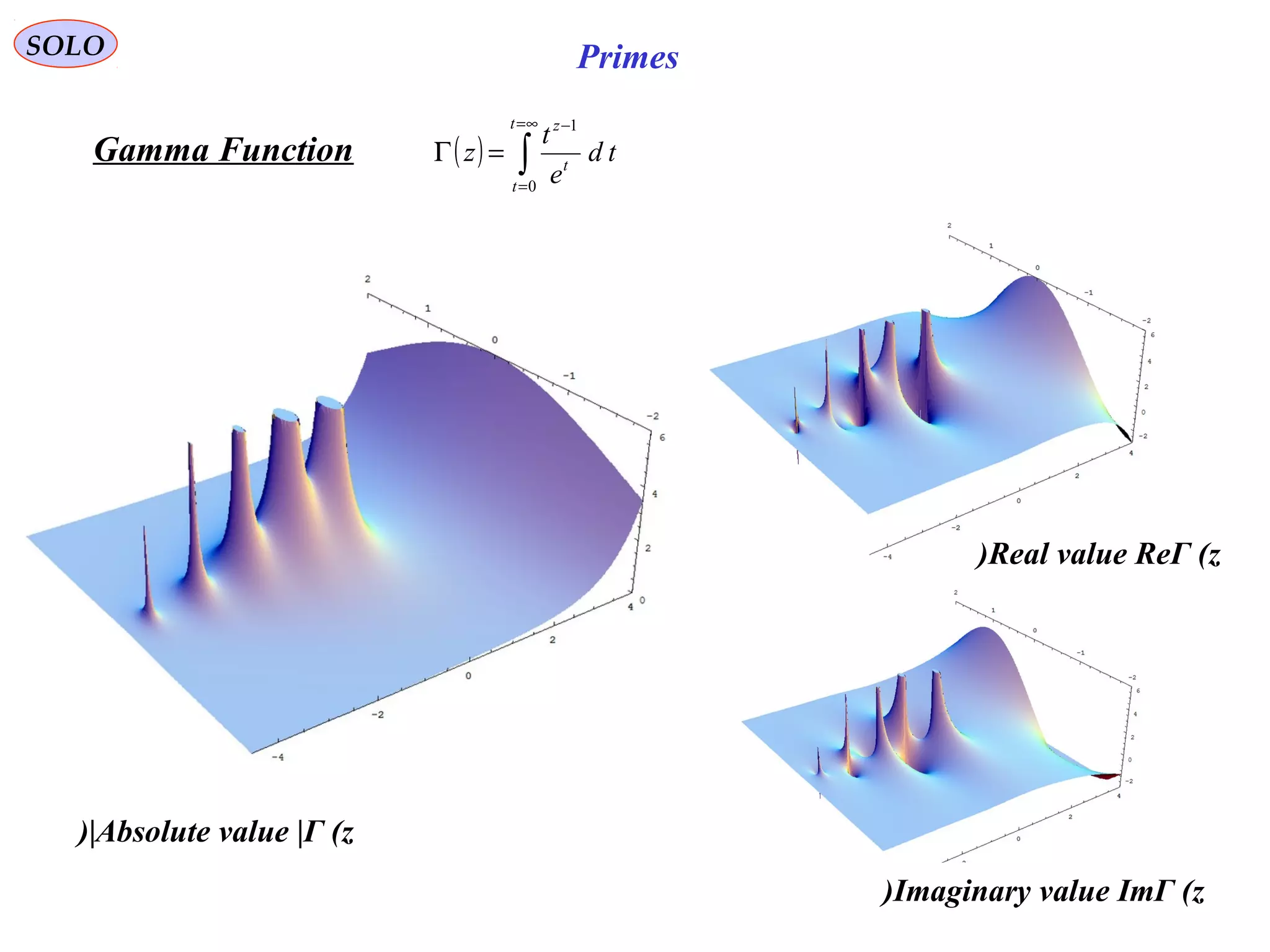
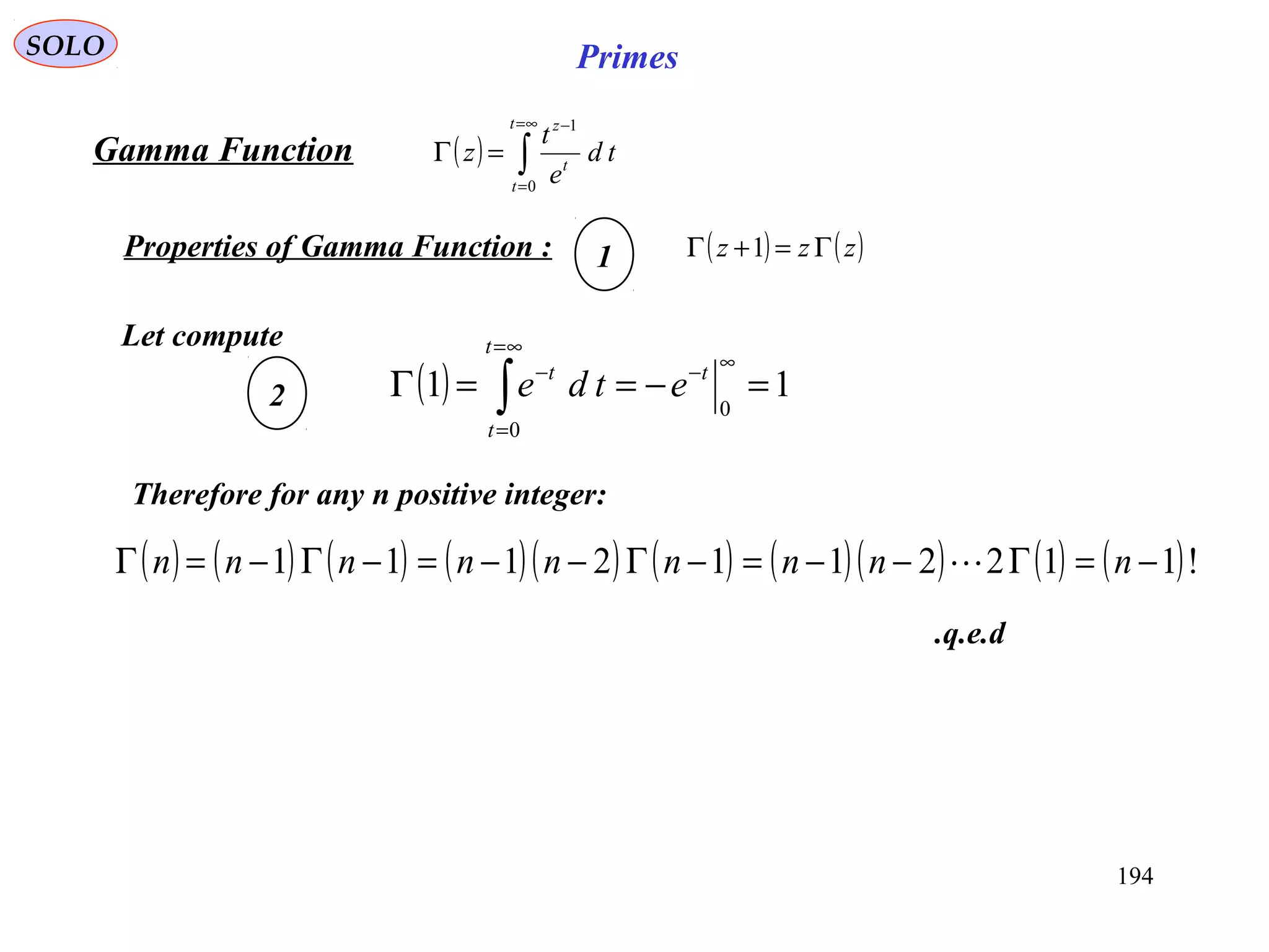
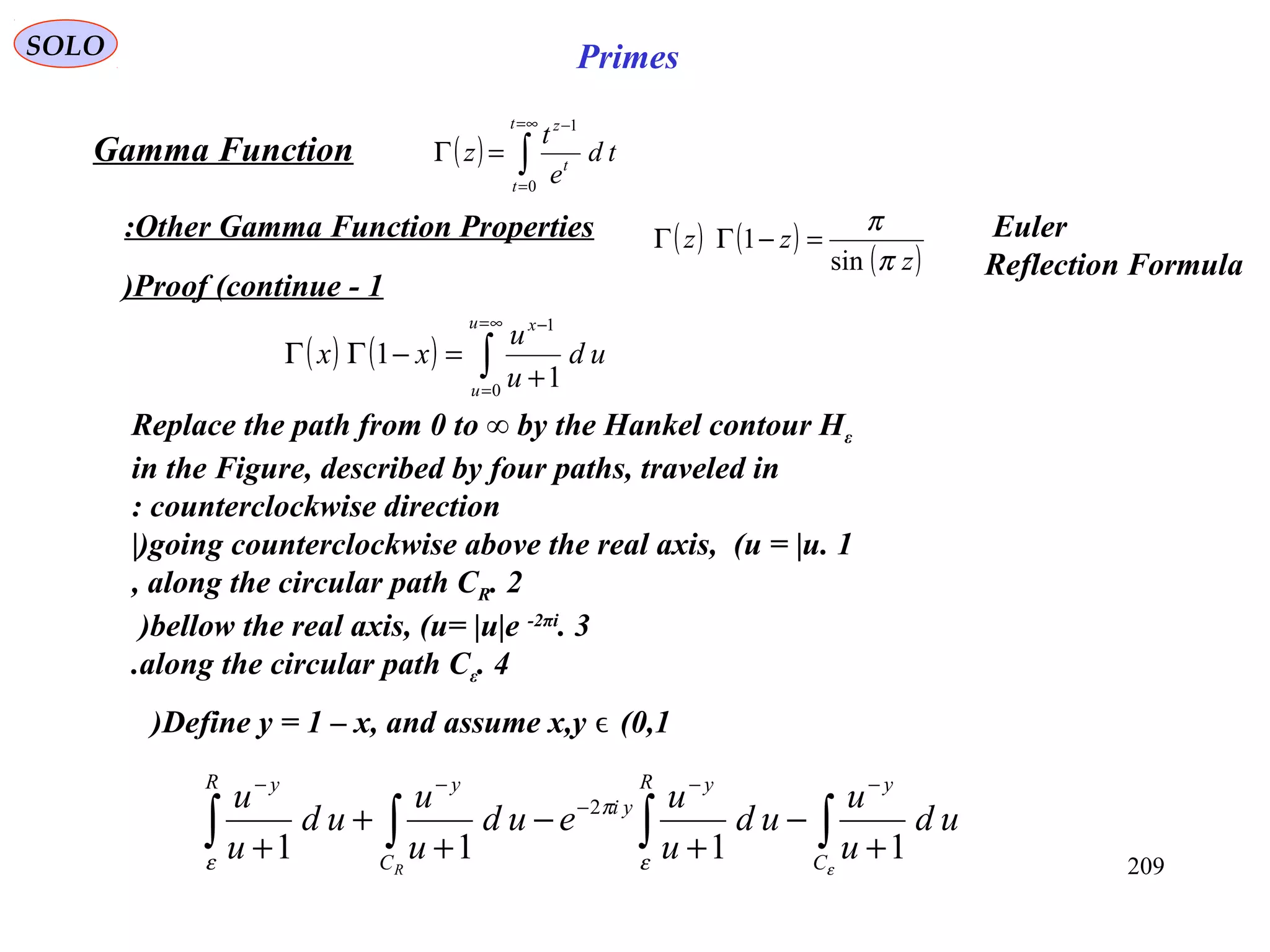
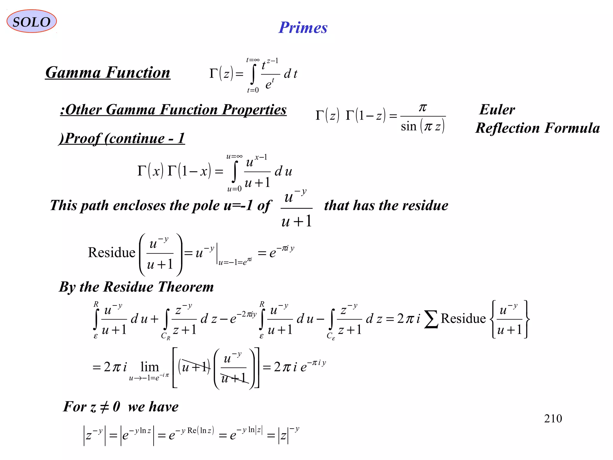
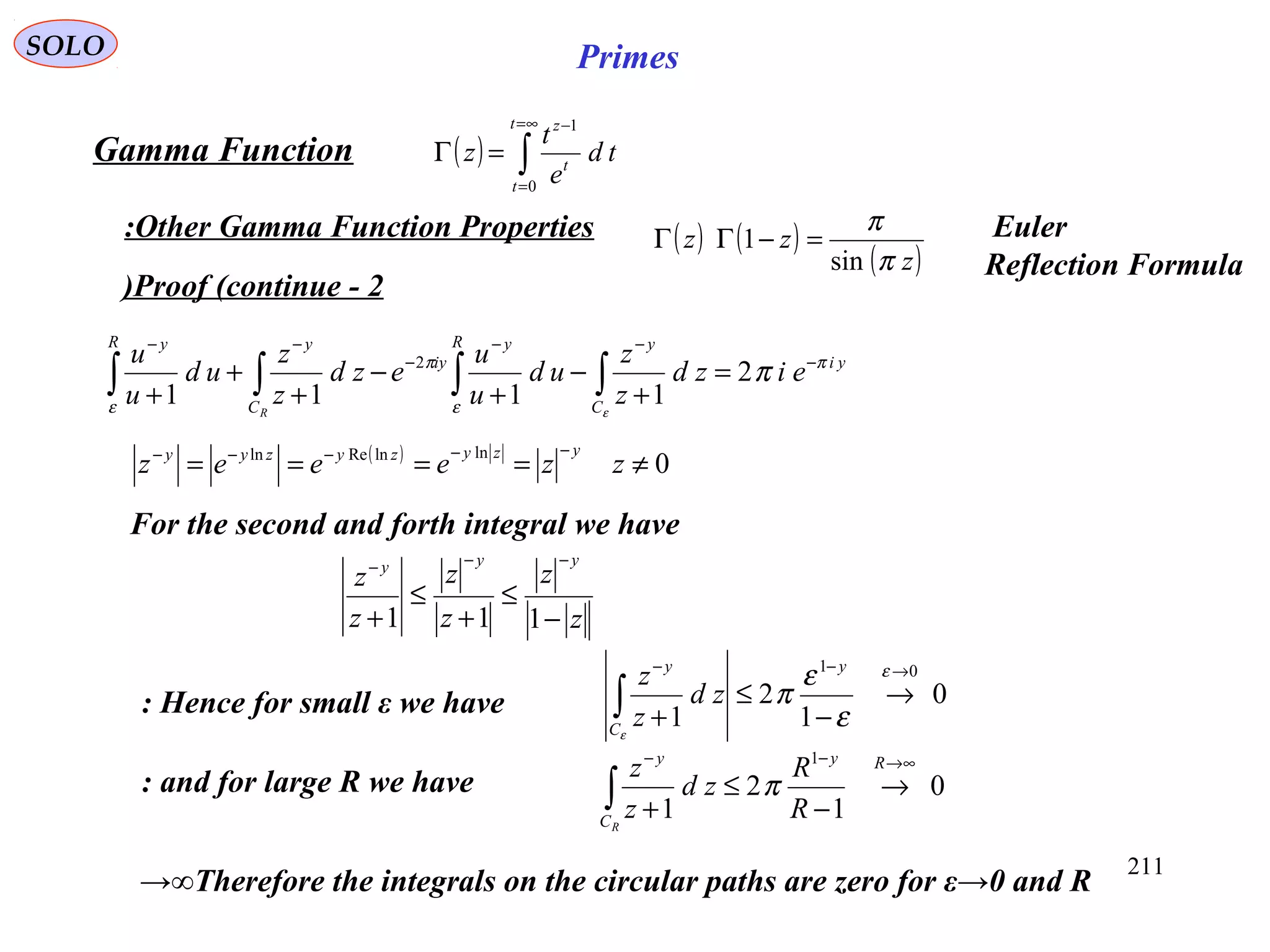
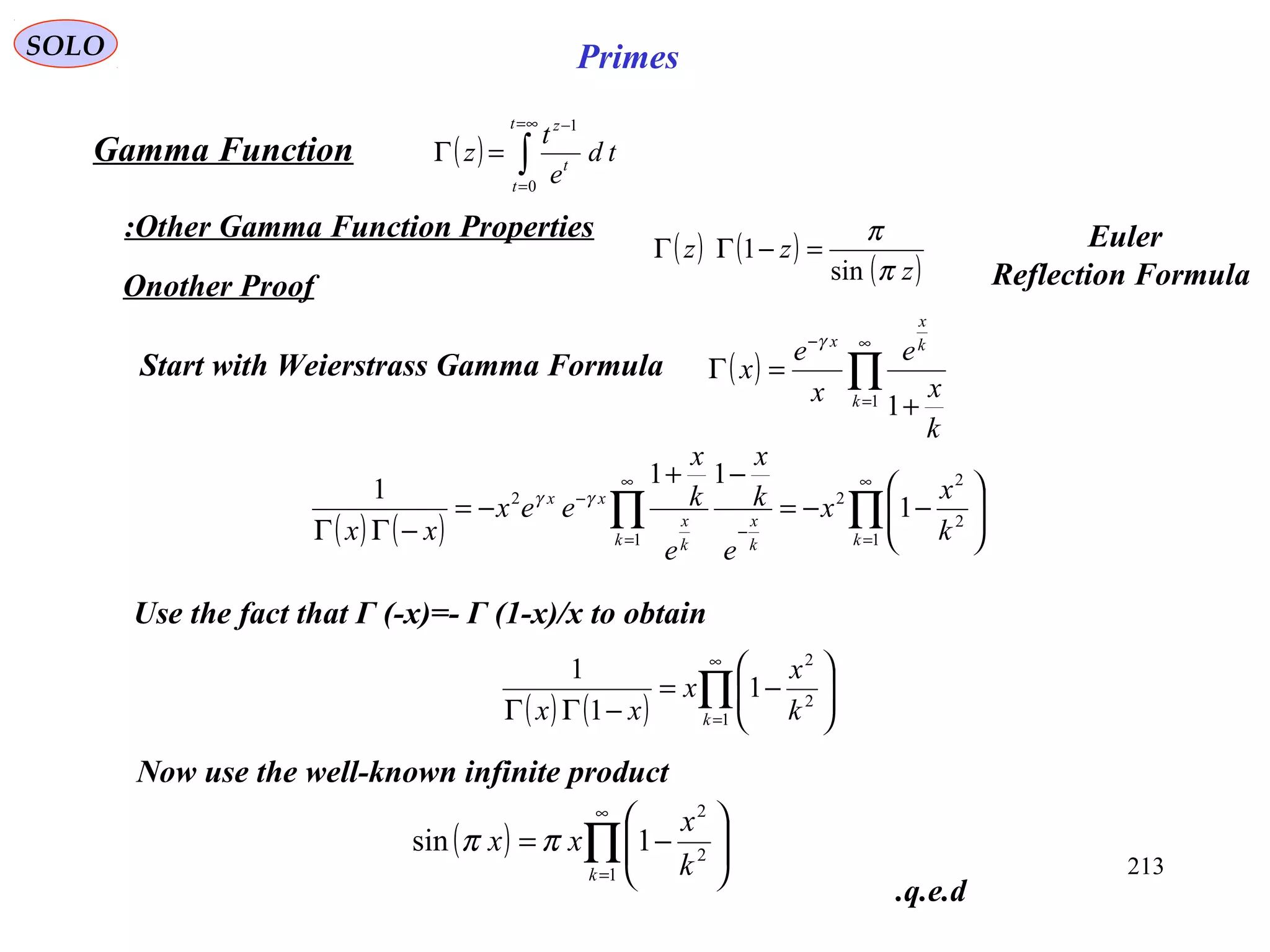
SOLO Primes
( ) ∫
∞=
=
−
=Γ
t
t
t
z
td
e
t
z
0
1
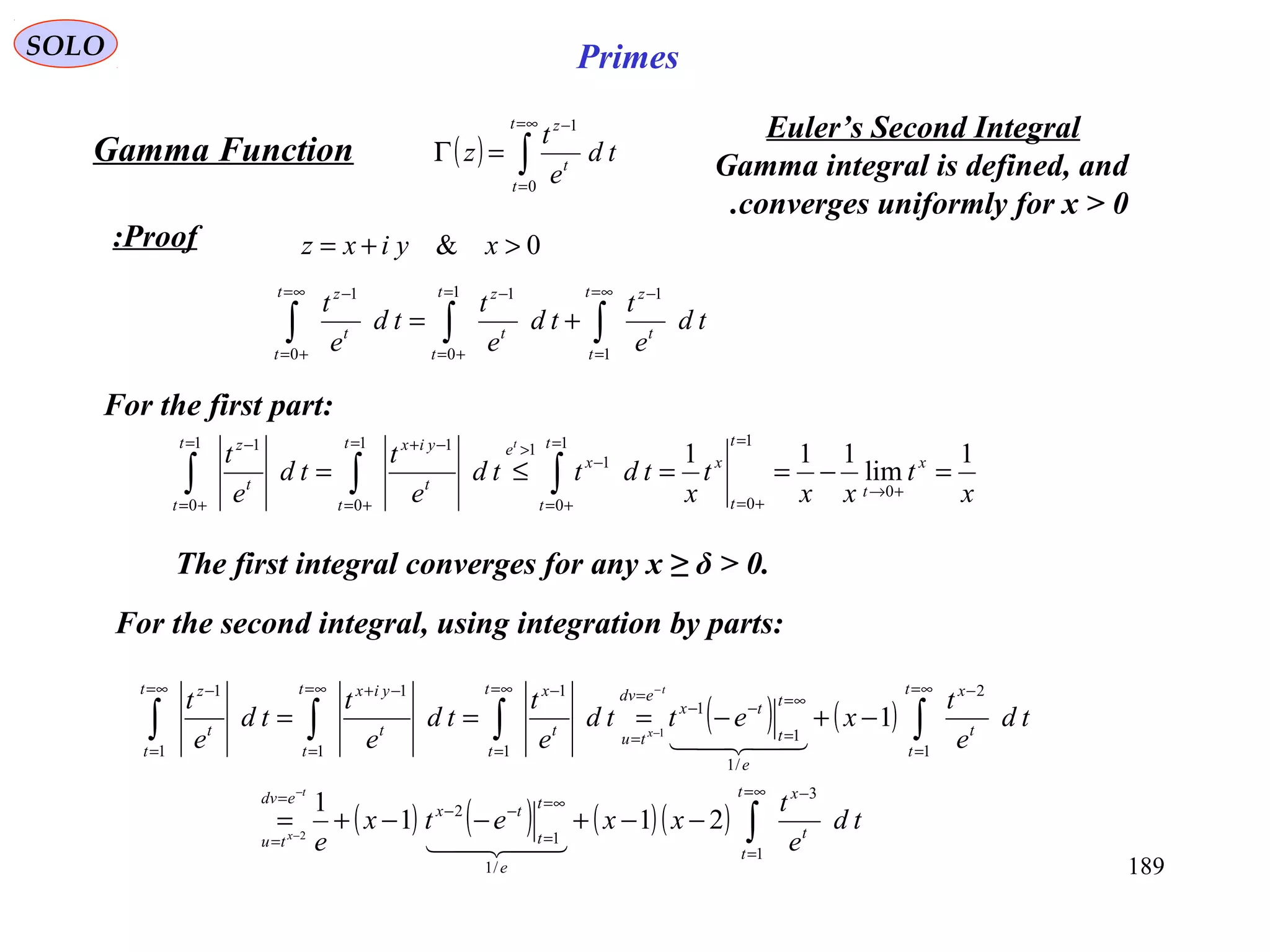
Proof (continue):
Gamma Function
0& >+= xyixz
For the second integral, using integration by parts:
( ) ( )
( ) ( ) ( )( ) ∫
∫∫∫∫
∞=
=
−
∞=
=
−−
=
=
∞=
=
−
∞=
=
−−
=
=
∞=
=
−∞=
=
−+∞=
=
−
−−+−−+=
−+−===
−
−
−
−
t
t
t
x
e
t
t
tx
edv
tu
t
t
t
x
e
t
t
tx
edv
tu
t
t
t
xt
t
t
yixt
t
t
z
td
e
t
xxetx
e
td
e
t
xettd
e
t
td
e
t
td
e
t
t
x
t
x
1
3
/1
1
2
1
2
/1
1
1
1
1
1
1
1
1
211
1
1
2
1
After [x] (the integer defined such that x-[x] < 1) such integration the power of t in
the integrand becomes x-[x]-1 < 0. and we have:
( )( ) [ ]( ) [ ]( ) ( )( ) [ ]( ) ∞<−−−<−−− ∫∫
∞=
=
∞=
=
−−
t
t
t
t
t
txx
td
e
xxxxtd
et
xxxx
11
1
1
21
1
21
Therefore the Gamma integral is defined, and converges uniformly for x > 0.
Gamma integral is defined, and
converges uniformly for x > 0.
q.e.d.](https://image.slidesharecdn.com/complexvariables-140921180830-phpapp02/75/Mathematics-and-History-of-Complex-Variables-190-2048.jpg)
![195
SOLO Primes
Second definition identical to First
( )[ ] ( ) ( ) ( ) ( ) ( )bayxallyfxfyxf ,,1,011 ∈∈−+≤−+ λλλλλ
Convex Function:
A Function f (x) is called Convex in an interval (a,b) if for every x,y (a,b) we haveϵ
A Function f (x), defined for x > 0, is called Convex, if the corresponding function
( ) ( ) ( )
y
xfyxf
y
−+
=φ
defined for all y > -x, y ≠ 0, is monotonic Increasing throughout the range of
definition.
If 0 < x1 < x < x2, are given by choosing y1 = x1 – x < 0, y2 = x2 – x > 0, we express
the condition of convexity as
( ) ( ) ( ) ( ) ( ) ( )
xx
xfxf
y
xx
xfxf
y
−
−
=≤
−
−
=
2
2
2
1
1
1 φφ
( ) ( )[ ] ( ) ( ) ( )[ ] ( )xxxfxfxxxfxf −−≥−− 1221
( ) ( ) ( )
( )
( ) ( )
( )
λλ −
−
−
+
−
−
≤
1
12
1
2
12
2
1
xx
xx
xf
xx
xx
xfxf
One other equivalent definition:](https://image.slidesharecdn.com/complexvariables-140921180830-phpapp02/75/Mathematics-and-History-of-Complex-Variables-195-2048.jpg)
![196
SOLO Primes
( )[ ] ( ) ( ) ( ) ( )1,0ln1ln1ln ∈−+≤−+ λλλλλ yfxfyxf
Logarithmic Convex Function :
A Function f (x)>0 is called logarithmic-convex or simply log-convex if ln (f (x) )
is convex or
This is equivalent to ( )[ ] ( ) ( )( )λλ
λλ
−
≤−+
1
ln1ln yfxfyxf
Since the logarithm is a momotonic increasing function we obtain
( )[ ] ( ) ( )( )
( ) yxyfxfyxf <∈≤−+
−
,1,01
1
λλλ
λλ](https://image.slidesharecdn.com/complexvariables-140921180830-phpapp02/75/Mathematics-and-History-of-Complex-Variables-196-2048.jpg)
![197
SOLO Primes
( ) ∫
∞=
=
−
=Γ
t
t
t
z
td
e
t
z
0
1
Proof :
Gamma Function
0& >+= xyixz
( )[ ] ( ) ( ) ( ) ( )1,0ln1ln1ln ∈Γ−+Γ≤−+Γ λλλλλ baba
Properties of Gamma Function :
3
Gamma is a
Log Convex
Function
( )[ ] ( )
( ) ( )
( ) ( ) λλ
λλ
λλλλ
λλ
−
−∞
−−
∞
−−
∞
−−−−−
∞
−−−+
ΓΓ=
≤
==−+Γ
∫∫
∫∫
1
1
0
1
0
1
0
111
0
11
1
badtetdtet
dtetetdtetba
tbta
InequalityHolder
tbtatba
q.e.d.](https://image.slidesharecdn.com/complexvariables-140921180830-phpapp02/75/Mathematics-and-History-of-Complex-Variables-197-2048.jpg)
![198
SOLO Primes
( ) ∫
∞=
=
−
=Γ
t
t
t
z
td
e
t
z
0
1
Proof :
Gamma Function
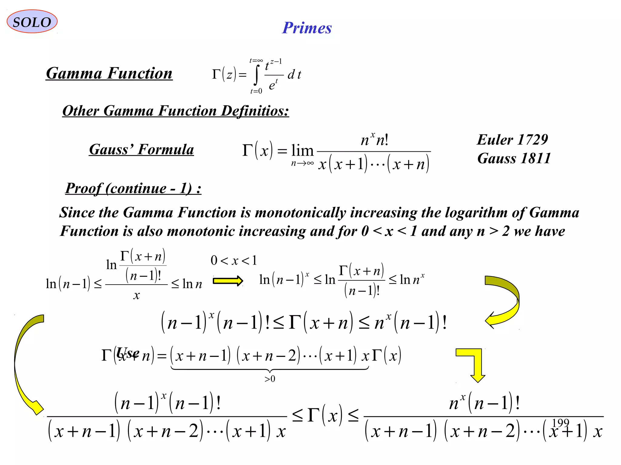
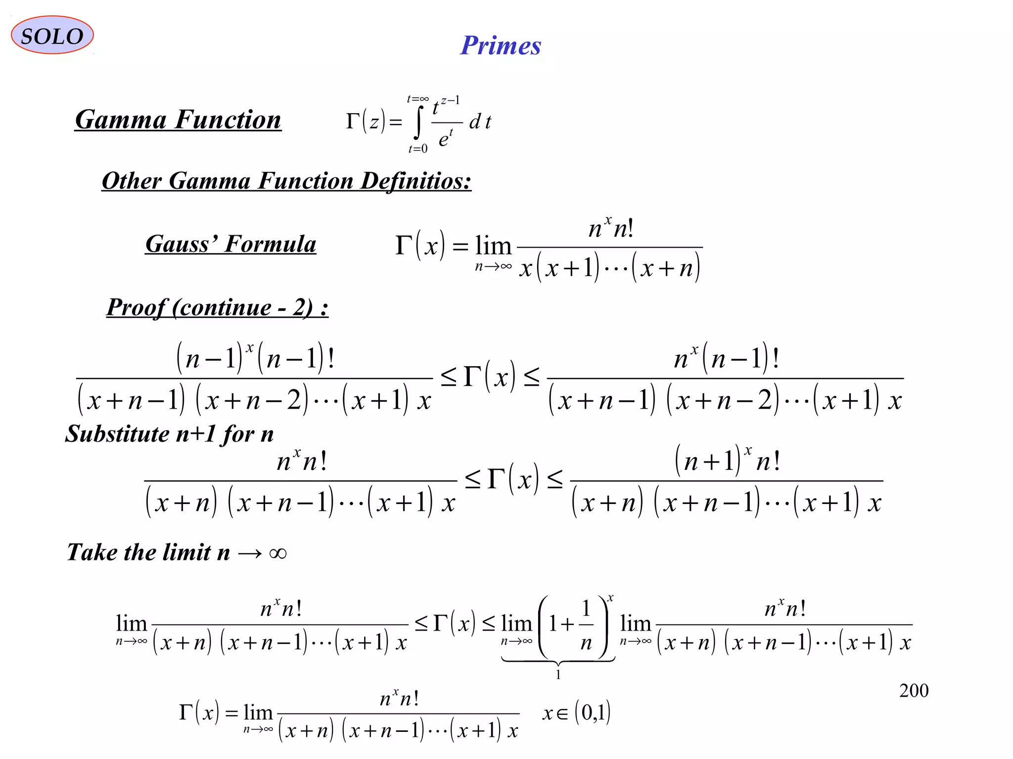
Other Gamma Function Definitios:
( )
( ) ( )nxxx
nn
x
x
n ++
=Γ
∞→ 1
!
limGauss’ Formula
Since the Gamma Function is monotonically increasing the logarithm of Gamma
Function is also monotonic increasing and for 0 < x < 1 and any n > 2 we have
( ) ( )
( ) nnx
nnx
−+
Γ−+Γ lnln
( )[ ] ( )[ ]
( )
( )
( ) ( )[ ] [ ] ( )[ ]
( )
−
−
−
−−
≤
−−+Γ
≤
−
−−−
!1
!
ln
!2
!1
ln
1
!1ln!ln!1lnln
1
!1ln!2ln
n
n
n
n
nn
x
nnxnn
( )
( )
( ) n
x
n
nx
n ln
!1
ln
1ln ≤
−
+Γ
≤−
( ) ( )
( )
1
1
ln1ln −=←
≤
−+−
Γ−+−Γ x
nn
nn ( ) ( )
( ) nn
nnx
−+
Γ−+Γ
≤
→=
1
ln1ln1
Carl Friedrich Gauss
(1777 – 1855)](https://image.slidesharecdn.com/complexvariables-140921180830-phpapp02/75/Mathematics-and-History-of-Complex-Variables-198-2048.jpg)
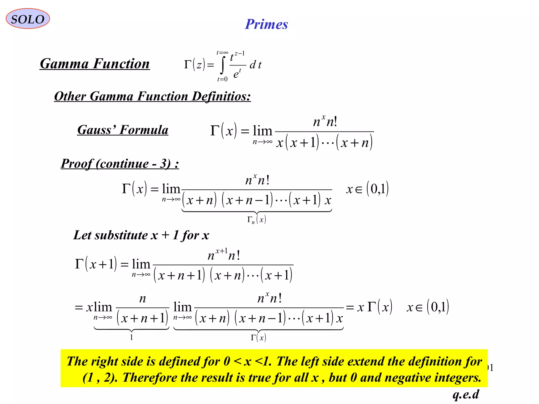
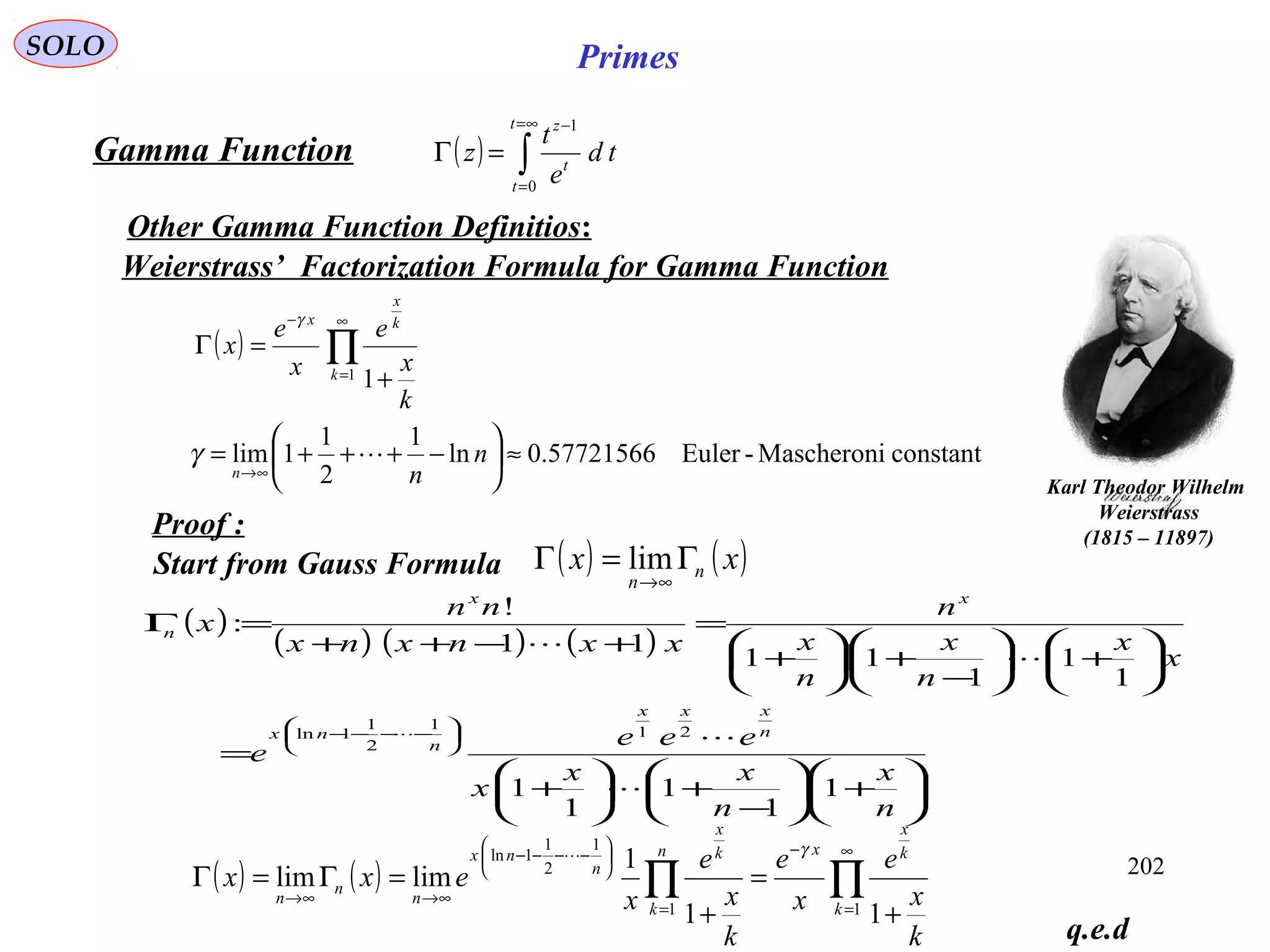
![212
SOLO Primes
Proof (continue - 3)
( ) ∫
∞=
=
−
=Γ
t
t
t
z
td
e
t
z
0
1
Gamma Function
Other Gamma Function Properties:
yi
y
iy
y
eiud
u
u
eud
u
u ππ
π −
∞ −
−
∞ −
=
+
−
+ ∫∫ 2
11 0
2
0
We obtain
Multiply both sides by yi
e π+
( ) iud
u
u
ee
y
iyiy
πππ
2
10
=
+
− ∫
∞ −
−
( ) ( )yee
i
ud
u
u
iyiy
y
π
π
π ππ
sin
2
10
=
−
=
+ −
∞ −
∫Rearranging we obtain
Since both sides of this equation are Holomorphic (analytic) in x (0,1) we canϵ
extend the result for all analytic parts of z C (complex planeϵ).
( ) ( )
( )[ ] ( )
( )1,0
sin1sin11
1
0
1
0
1
∈=
−
=
+
=
+
=−ΓΓ ∫∫
∞=
=
−−=∞=
=
−
x
xx
ud
u
u
ud
u
u
xx
u
u
yxyu
u
x
π
π
π
π
Substituting y = 1 – x we obtain
( ) ( )
( )z
zz
π
π
sin
1 =−ΓΓ Euler
Reflection Formula](https://image.slidesharecdn.com/complexvariables-140921180830-phpapp02/75/Mathematics-and-History-of-Complex-Variables-212-2048.jpg)

![233
SOLO
Proof (continue – 2): 0& >+= xyixz
( ) ∫∫∫
∞=
=
−=
+=
−∞=
=
−
−
+
−
=
−
=
++Γ
t
t
t
zt
t
t
zt
t
t
z
zz
td
e
t
td
e
t
td
e
t
z
φ
φ
ln2
1ln2
0
1
0
1
1112
1
1
1
In the second integral we have
This integral converges only for x > 1, therefore we proved that
φln21 2/
≥≥− tforee tt
since RatioGoldeneforee ttt
==
+
≥≥−− φ
2
51
01 2/2/
( ) ( )( ) ∫∫∫∫
∞=
=
−
∞
=
−−
=
=
∞=
=
−∞=
=
−+=∞=
=
−
−−−−=≤
−
=
−
−
−
t
t
t
x
termfinite
t
tx
tu
dtedv
t
t
t
xt
t
t
xiyxzt
t
t
z
td
e
t
xettd
e
t
td
e
t
td
e
t
x
t
φ
φ
φφφ ln2
2/
2
ln2
2/1
ln2
2/
1
ln2
1
ln2
1
122
11
1
2/
( ) [ ]
( )( ) [ ]( ) [ ]( ) ∞<−−−−−= ∫∑∫
∞=
=
−−
−
∞=
=
−
finite
t
t
txx
xx
t
t
t
x
td
et
xxxxtermsfinitetd
e
t
φφ ln2
2/1
ln2
2/
1
1
212
( ) ( ) ( ) ( ) 1Re
12
1
1
1
0
1
>=∞<
−
=Γ=
++Γ ∫
∞=
=
−
zxfortd
e
t
zzz
t
t
t
z
zz
ς
( ) ( ) ( ) 1Re
10
1
>=∞<
−
=Γ ∫
∞=
=
−
zxfordt
e
t
zz
t
t
t
z
ς
After [x] (the integer defined such that x-[x] < 1) such integration the power of t in
the integrand becomes x-[x]-1 < 0. and we have:
q.e.d.
Riemann's Zeta Function](https://image.slidesharecdn.com/complexvariables-140921180830-phpapp02/75/Mathematics-and-History-of-Complex-Variables-233-2048.jpg)
![235
SOLO
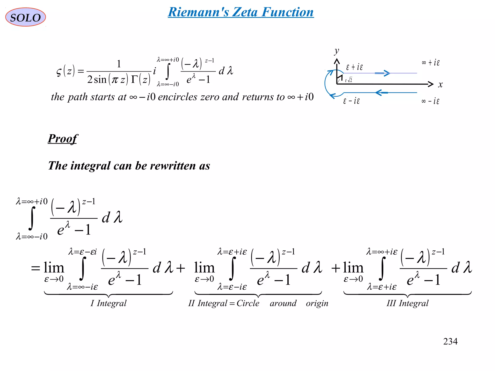
Proof (continue – 1)
The first integral can be written as
εi−∞
εi+∞
y
x
εε i+
εε i−
2ε
( ) ( )[ ] ( )
∫∫∫∫
∞=
+=
−
−
−=+=
∞=
−
−−
=
∞=
−
−−
→
−=−=
−∞=
−
→ −
=
−
=
−
−
=
−
−
− t
t
t
z
zi
et
t
t
z
zi
t
t
it
ziiti
i
z
td
e
t
etd
e
t
etd
e
eit
d
e
i
0
110 1
1
1
0
0 1
0 111
lim
1
lim ππ
ε
ε
π
ε
ελεελ
ελ
λε
π
ε
λ
λ
The second integral can be written as
( ) ( )
( ) ( ) 0
1
2
lim2
1
2
lim
2
1
2
lim
1
lim
2
0
20
2
0
2
1
0
2
0
2
1
0
21
0
→
−
=
−
−
≤
−
−
=
−
−
∫∫
∫∫
=
=
→
=
=
−+
→
=
=
−+
→
=+=
−=
−
→
πθ
θ
εε
πθ
θ
θ
ε
θ
ε
πθ
θ
θ
ε
θ
ε
ελεελ
εελ
λε
θ
ε
θε
ε
θε
ε
λ
λ
θθ
θ
θ
d
e
dei
e
e
dei
e
e
d
e
ii
i
i
e
x
i
e
iyxi
i
e
iyxie
originaroundCircle
i
i
z
( )
( ) ( )
( )
00
1sin2
1
0
0
1
itoreturnsandzeroencirclesiatstartspaththe
d
e
i
zz
z
i
i
z
+∞−∞
−
−
Γ
= ∫
+∞=
−∞=
−λ
λ
λ
λ
λ
π
ς
Riemann's Zeta Function](https://image.slidesharecdn.com/complexvariables-140921180830-phpapp02/75/Mathematics-and-History-of-Complex-Variables-235-2048.jpg)
![236
SOLO
Proof (continue – 2)
The third integral can be written as
εi−∞
εi+∞
y
x
εε i+
εε i−
2ε
( ) ( )[ ] ( )
∫∫∫∫
∞=
+=
−−=∞=
+=
−
−
∞=
=
+
−
→
+=+∞=
+=
−
→ −
−=
−
=
−
+
=
−
−
− t
t
t
z
zi
et
t
t
z
zi
t
t
it
ziiti
i
z
td
e
t
etd
e
t
etd
e
eit
d
e
i
0
11
0
1
1
1
0
1
0 111
lim
1
lim ππ
ε
ε
π
ε
ελελ
εελ
λε
π
ε
λ
λ
Therefore
( ) ( ) ( ) ( ) ∫∫∫∫
∞=
+=
−∞=
+=
−−∞=
+=
−
−
+∞=
−∞=
−
−
−=
−
−
−=
−
−=
−
−
t
t
t
zt
t
t
zzizit
t
t
z
zizi
i
i
z
td
e
t
zitd
e
t
i
ee
itd
e
t
eed
e 0
1
0
1
0
10
0
1
1
sin2
12
2
11
πλ
λ ππ
ππ
λ
λ
λ
But we found that ( ) ( ) ( ) 1Re
10
1
>=∞<
−
=Γ ∫
∞=
=
−
zxfordt
e
t
zz
t
t
t
z
ς
( )
( ) ( )
( )
00
1sin2
1
0
0
1
itoreturnsandzeroencirclesiatstartspaththe
d
e
i
zz
z
i
i
z
+∞−∞
−
−
Γ
= ∫
+∞=
−∞=
−λ
λ
λ
λ
λ
π
ς
Therefore ( )
( ) ( )
( )
∫
+∞=
−∞=
−
−
−
Γ
=
0
0
1
1sin2
1
i
i
z
d
e
i
zz
z
λ
λ
λ
λ
λ
π
ς
The right hand is analytic for any z ≠ 1. Since it equals Zeta Function in the half
plane x > 1, it is the Analytic Continuation of Zeta to the complax plane for any z ≠ 1.
( )
( ) ( )
( )
∫
+∞=
−∞=
−
−
−
Γ
=
0
0
1
1sin2
1
i
i
z
d
e
i
zz
z
λ
λ
λ
λ
λ
π
ς q.e.d.
Riemann's Zeta Function](https://image.slidesharecdn.com/complexvariables-140921180830-phpapp02/75/Mathematics-and-History-of-Complex-Variables-236-2048.jpg)
![238
SOLO
Proof (continue)
( ) ( ) ( )∫
+∞=
−∞=
−
−
−=
−
−
0
0
1
1
2
sin22
1
i
i
z
z
z
z
id
e
λ
λ
λ
ς
π
πλ
λ
( ) ( ) ( ) ( ) ( )[ ] ∑∑∑∫
∞
=
−
−−
∞
=
−
∞
=
−
+∞
−∞
−
+−=+−=
−
−
1
1
11
1
1
1
1
0
0
1
1
22222
1 n
z
zzz
n
z
n
z
i
i
z
n
iiiniiniid
e
πππππλ
λ
λ
( )[ ] ( ) ( ) ( )
[ ] ( ) ( )
[ ]
−=−=−=−−=+− −−−−
2
sin22/2/lnln11 z
eeieeiiiiiii izizizizzzzz πππ
( )z
nn
z
−=∑
∞
=
−
1
1
1
1
ς
( ) ( ) ( )z
z
id
e
z
i
i
z
−
−=
−
−
∫
+∞
−∞
−
1
2
sin22
1
0
0
1
ς
π
πλ
λ
λ
q.e.d.
Riemann's Zeta Function](https://image.slidesharecdn.com/complexvariables-140921180830-phpapp02/75/Mathematics-and-History-of-Complex-Variables-238-2048.jpg)
![242
SOLO
Proof
Start from
use
( ) ( ) ( ) ( ) ( )z
z
zzz
z
−
=Γ 1
2
sin22sin2 ς
π
πςπ
( ) ( )
( )z
zz
π
π
sin
1 =−ΓΓ
( ) ( )
( )z
zz
−Γ
=Γ
1
sin
π
π
−Γ
Γ
=
2
1
2
2
sin
zz
z π
π
z
z
→
2
( )
( ) ( )
( ) ( )
( )z
z
zz
z
z
z
−
−ΓΓ
=
−Γ
1
2
sin
2/12/
1
2
1
1
ς
π
πς
or
( ) ( ) ( )
( )
( )
( )z
z
zzz zzz
−
−Γ
−Γ=Γ −−−
1
2/1
1
122/ 2/12/12/
ςππςπ
( ) ( )
( )
( )
( )[ ] ( )
( )
z
z
z
z
zzzz
−
−−−
−−Γ=Γ
1
2/12/
12/12/
ηη
ςπςπ
Riemann's Zeta Function](https://image.slidesharecdn.com/complexvariables-140921180830-phpapp02/75/Mathematics-and-History-of-Complex-Variables-242-2048.jpg)
![243
SOLO
Proof (continue)
( ) ( )
( )
( )
( )[ ] ( )
( )
z
z
z
z
zzzz
−
−−−
−−Γ=Γ
1
2/12/
12/12/
ηη
ςπςπ
or
( ) ( ) ( )
( )
( )
( )z
z
zzz zzz
−
−Γ
−Γ=Γ −−−
1
2/1
1
122/ 2/12/12/
ςππςπ
( )
+
Γ
Γ=Γ −−
2
1
2
2 12/1 zz
z z
π
( ) ( )2/1
2
1
21 2/1
z
z
z z
−Γ
−
Γ=−Γ −−
π z
z
−
↓
1
( )
( )
−
Γ=
−Γ
−Γ
2
1
2/1
1
122/1 z
z
zz
π
therefore
q.e.d.
( ) ( ) ( )
( )z
z
zz zz
−
−
Γ=Γ −−−
1
2
1
2/ 2/12/
ςπςπ
Use Legendre
Duplication Formula: ( ) ( ) 0Re2
22
1
12
>Γ=
+ΓΓ −
zzzz z
π
2/z
z
↓
Riemann's Zeta Function](https://image.slidesharecdn.com/complexvariables-140921180830-phpapp02/75/Mathematics-and-History-of-Complex-Variables-243-2048.jpg)
![246
SOLO
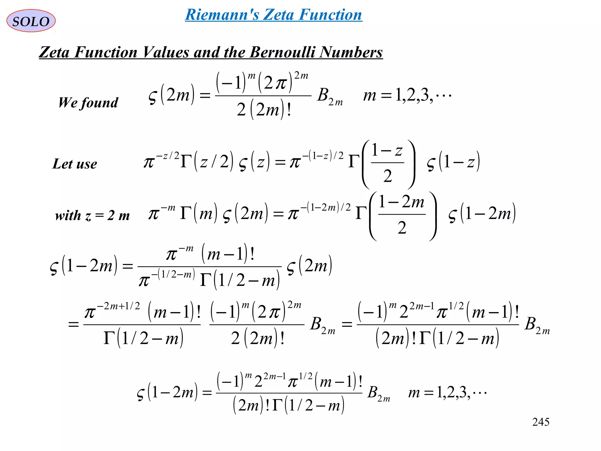
Zeta Function Values and the Bernoulli Numbers
We found
( ) ( )
( )
( ) ( )[ ]
( ) ( )[ ]
( ) ( )
( )
2/1
12
2/1
1
2/1
!12
!121
224212531
121221
12531
21
2/1
π
ππ
⋅
−
−⋅−
=
⋅
−⋅⋅−⋅⋅
−⋅⋅⋅−
=
−⋅⋅
−
=+−Γ
−
−
m
m
mm
m
m
m
mm
mmmmm
( ) ( ) ( )
( ) ( )
,3,2,1
2/1!2
!121
21 2
2/112
=
+−Γ
−−
=−
−
mB
mm
m
m m
mm
π
ςTherefore
Finally
( ) ( )
( )
,2,1,0
1
1 1
=
+
−−=− +
n
n
B
n nn
ς
( ) ,3,2,1
2
1
21 2 ==− mB
m
m mς
We also found The two expressions
Agree.
Riemann Zeta Function
Riemann's Zeta Function](https://image.slidesharecdn.com/complexvariables-140921180830-phpapp02/75/Mathematics-and-History-of-Complex-Variables-246-2048.jpg)
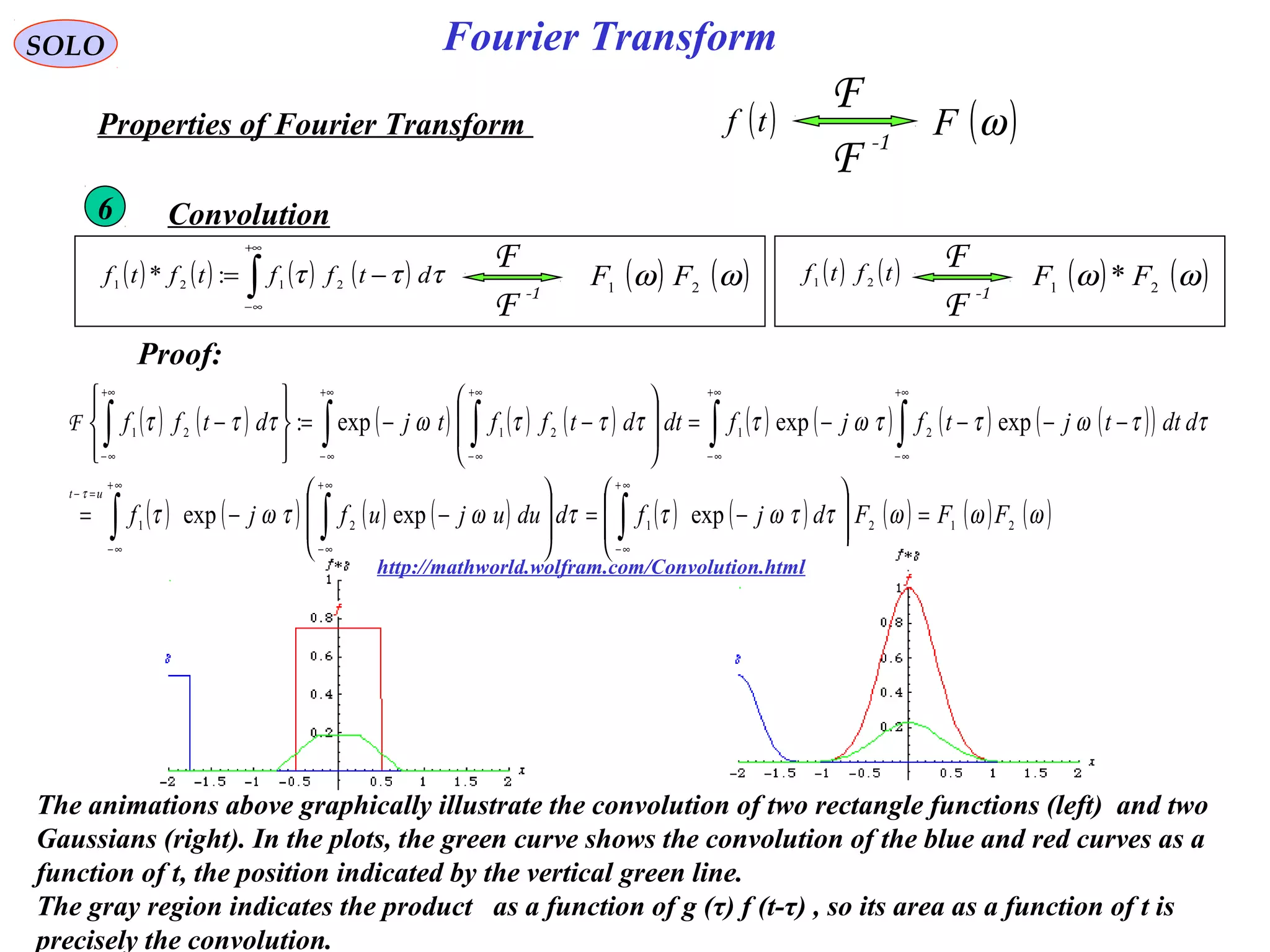
![Fourier Transform
( ) ( ){ } ( ) ( )∫
+∞
∞−
−== dttjtftfF ωω exp:F
SOLO
Jean Baptiste Joseph
Fourier
1768 - 1830
F (ω) is known as Fourier Integral or Fourier Transform
and is in general complex
( ) ( ) ( ) ( ) ( )[ ]ωφωωωω jAFjFF expImRe =+=
Using the identities
( ) ( )t
d
tj δ
π
ω
ω =∫
+∞
∞− 2
exp
we can find the Inverse Fourier Transform ( ) ( ){ }ωFtf -1
F=
( ) ( ) ( ) ( ) ( )
( ) ( )( ) ( ) ( ) ( ) ( )[ ]00
2
1
2
exp
2
expexp
2
exp
++−=−=−=
−=
∫∫ ∫
∫ ∫∫
∞+
∞−
∞+
∞−
∞+
∞−
+∞
∞−
+∞
∞−
+∞
∞−
tftfdtfd
d
tjf
d
tjdjf
d
tjF
ττδττ
π
ω
τωτ
π
ω
ωττωτ
π
ω
ωω
( ) ( ){ } ( ) ( )∫
+∞
∞−
==
π
ω
ωωω
2
exp:
d
tjFFtf -1
F
( ) ( ) ( ) ( )[ ]00
2
1
++−=−∫
+∞
∞−
tftfdtf ττδτ
If f (t) is continuous at t, i.e. f (t-0) = f (t+0)
This is true if (sufficient not necessary)
f (t) and f ’ (t) are piecewise continue in every finite interval1
2 and converge, i.e. f (t) is absolute integrable in (-∞,∞)( )∫
+∞
∞−
dttf](https://image.slidesharecdn.com/complexvariables-140921180830-phpapp02/75/Mathematics-and-History-of-Complex-Variables-249-2048.jpg)
![Fourier TransformSOLO
( )tf
-1
F
F
( )ωFProperties of Fourier Transform
Linearity1
( ) ( ){ } ( ) ( )[ ] ( ) ( ) ( )ωαωαωαααα 221122112211 exp: FFdttjtftftftf +=−+=+ ∫
+∞
∞−
F
Symmetry2
( )tF
-1
F
F
( )ωπ −f2
( ) ( ) ( ) ( ) ( ) ( ) ( ) ( ) ( ) ( ){ }tFdttjtFf
dt
tjtFf
d
tjFtf
t
F=−=−⇒=⇒= ∫∫∫
+∞
∞−
+∞
∞−
↔
+∞
∞−
ωωπ
π
ωω
π
ω
ωω
ω
exp2
2
exp
2
exp
Proof:
Conjugate Functions3
( )tf *
-1
F
F
( )ω−*
F
Proof:
( ) ( ) ( ) ( ) ( ) ( ){ }tf
d
tjF
d
tjFtf ****
2
exp
2
exp 1-
F=−=−= ∫∫
+∞
∞−
→−
+∞
∞−
π
ω
ωω
π
ω
ωω
ωω](https://image.slidesharecdn.com/complexvariables-140921180830-phpapp02/75/Mathematics-and-History-of-Complex-Variables-250-2048.jpg)
![Fourier TransformSOLO
( )tf
-1
F
F
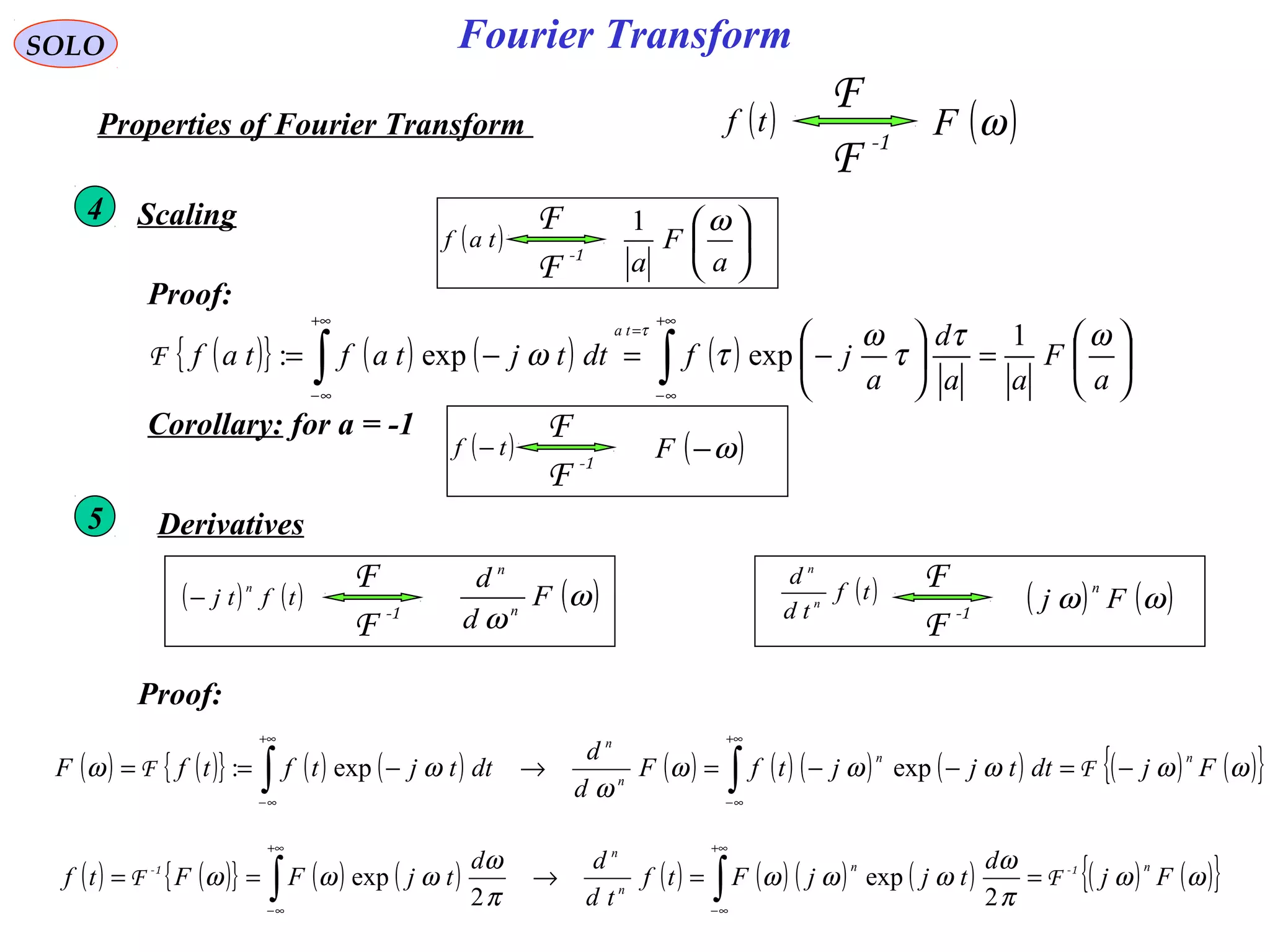
( )ωFProperties of Fourier Transform
Modulation9
Shifting: for any a real8
Proof:
( ) ttf 0cos ω -1
F
F
( ) ( )[ ]00
2
1
ωωωω −++ FF
Proof:
( ) ( )[ ]tjtjt 000 expexp
2
1
cos ωωω −+=
( )atf −
-1
F
F ( ) ( )ωω ajF −exp ( ) ( )tajtf exp
-1
F
F ( )aF −ω
( ){ } ( ) ( ) ( ) ( )( ) ( ) ( )ωωττωτω
τ
Fajdajfdttjatfatf
at
−=+−=−−=− ∫∫
+∞
∞−
=−
+∞
∞−
expexpexp:F
( ) ( ){ } ( ) ( ) ( ) ( ) ( )( ) ( )aFdttajtfdttjtajtftajtf −=−−=−= ∫∫
+∞
∞−
+∞
∞−
ωωω expexpexp:expF
use shifting property with a=±ω0](https://image.slidesharecdn.com/complexvariables-140921180830-phpapp02/75/Mathematics-and-History-of-Complex-Variables-255-2048.jpg)
![( )atf −
-1
F
F ( ) ( )ωω ajF −exp
Fourier TransformSOLO
( )tf
-1
F
F
( )ωFProperties of Fourier Transform (Summary)
Linearity1
( ) ( ){ } ( ) ( )[ ] ( ) ( ) ( )ωαωαωαααα 221122112211 exp: FFdttjtftftftf +=−+=+ ∫
+∞
∞−
F
Symmetry2
( )tF
-1
F
F
( )ωπ −f2
Conjugate Functions3 ( )tf *
-1
F
F
( )ω−*
F
Scaling4 ( )taf
-1
F
F
a
F
a
ω1
Derivatives5 ( ) ( )tftj
n
−
-1
F
F ( )ω
ω
F
d
d
n
n
( )tf
td
d
n
n
-1
F
F
( ) ( )ωω Fj
n
Convolution6
( ) ( )tftf 21
-1
F
F ( ) ( )ωω 21
* FF( ) ( ) ( ) ( )∫
+∞
∞−
−= τττ dtfftftf 2121
:*
-1
F
F ( ) ( )ωω 21
FF
( ) ( ) ( ) ( )∫∫
+∞
∞−
+∞
∞−
= ωωω
π
dFFdttftf 2
*
12
*
1
2
1
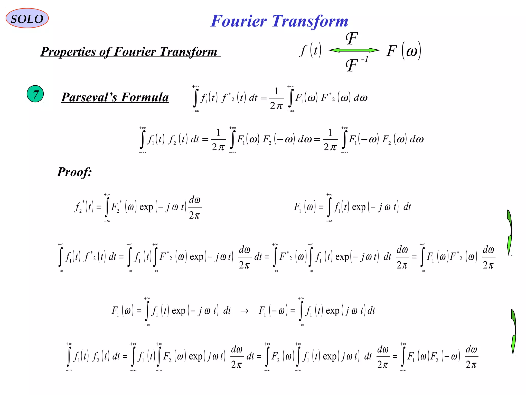
Parseval’s Formula7
Shifting: for any a real8
( ) ( )tajtf exp
-1
F
F ( )aF −ω
Modulation9 ( ) ttf 0
cos ω -1
F
F
( ) ( )[ ]00
2
1
ωωωω −++ FF
( ) ( ) ( ) ( ) ( ) ( )∫∫∫
+∞
∞−
+∞
∞−
+∞
∞−
−=−= ωωω
π
ωωω
π
dFFdFFdttftf 212121
2
1
2
1](https://image.slidesharecdn.com/complexvariables-140921180830-phpapp02/75/Mathematics-and-History-of-Complex-Variables-256-2048.jpg)
![( ) ( ){ } ( ) ( )∫
+∞
∞−
−== dttjtftfF νπνπ 2exp:2 F
( ) ( ) ( )∑∑
∞
=
−
+∞
−∞=
=
+=
0
* 21
n
nsT
n
eTnf
T
n
jsF
T
sF
π
( ) ( ){ } ( ) ( )∫
+∞
∞−
== ννπνπνπ dtjFFtf 2exp2:2-1
F
SOLO
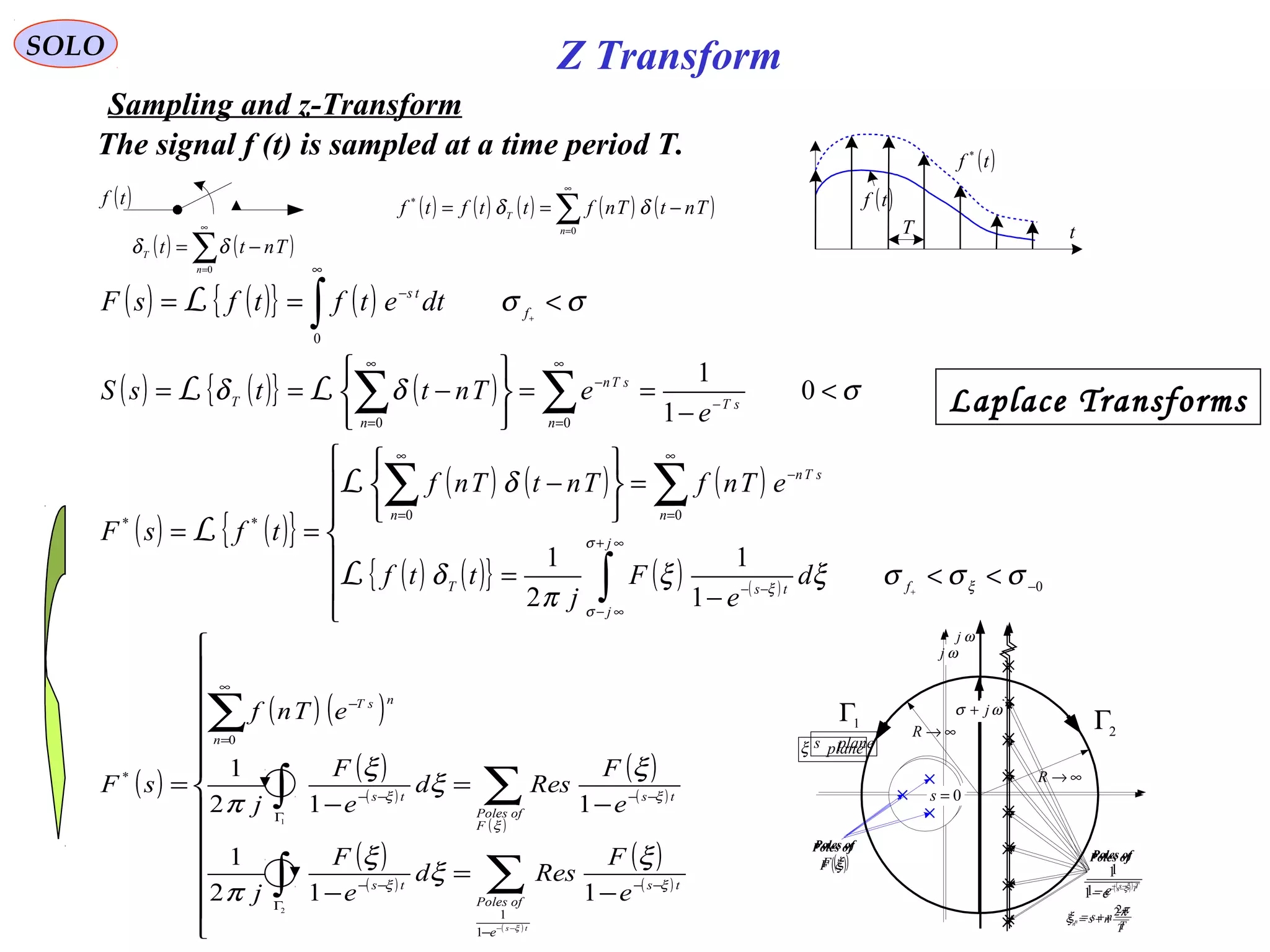
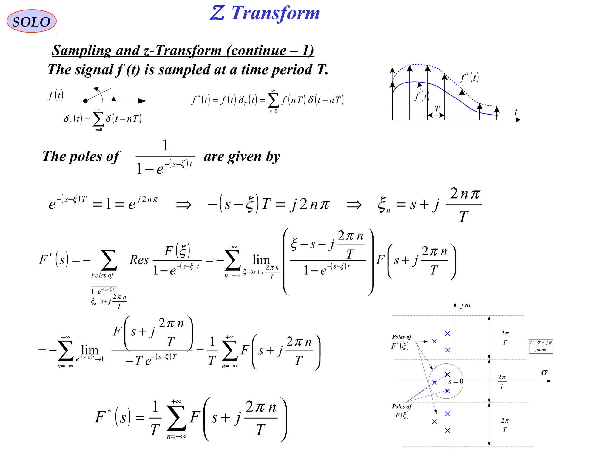
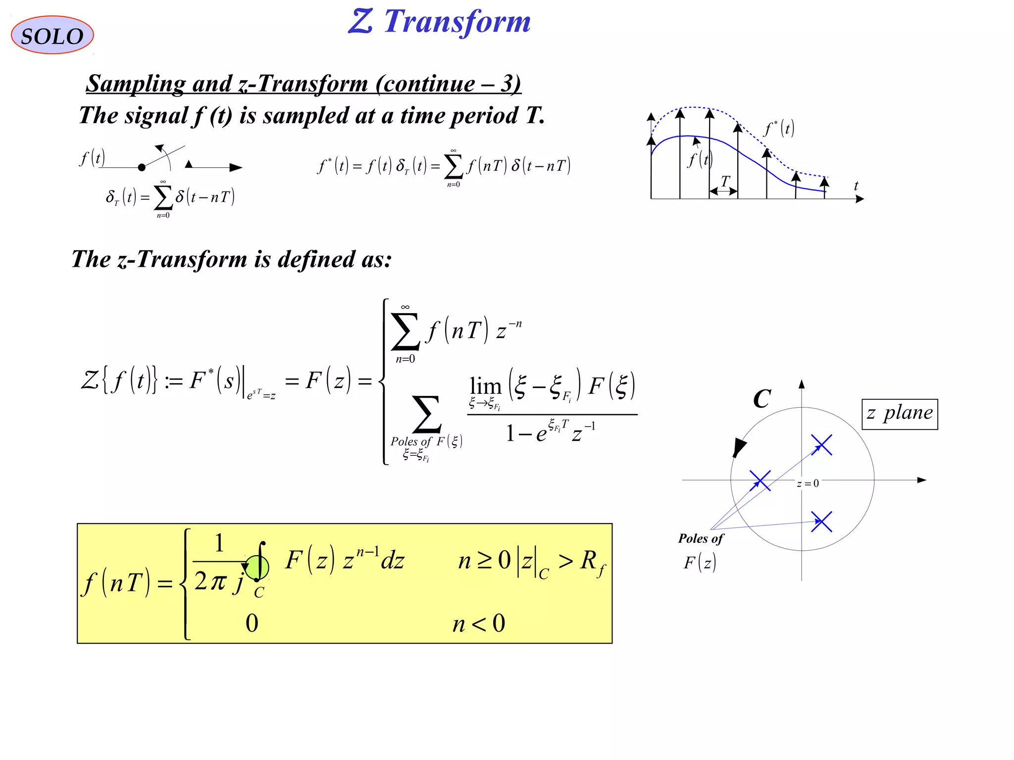
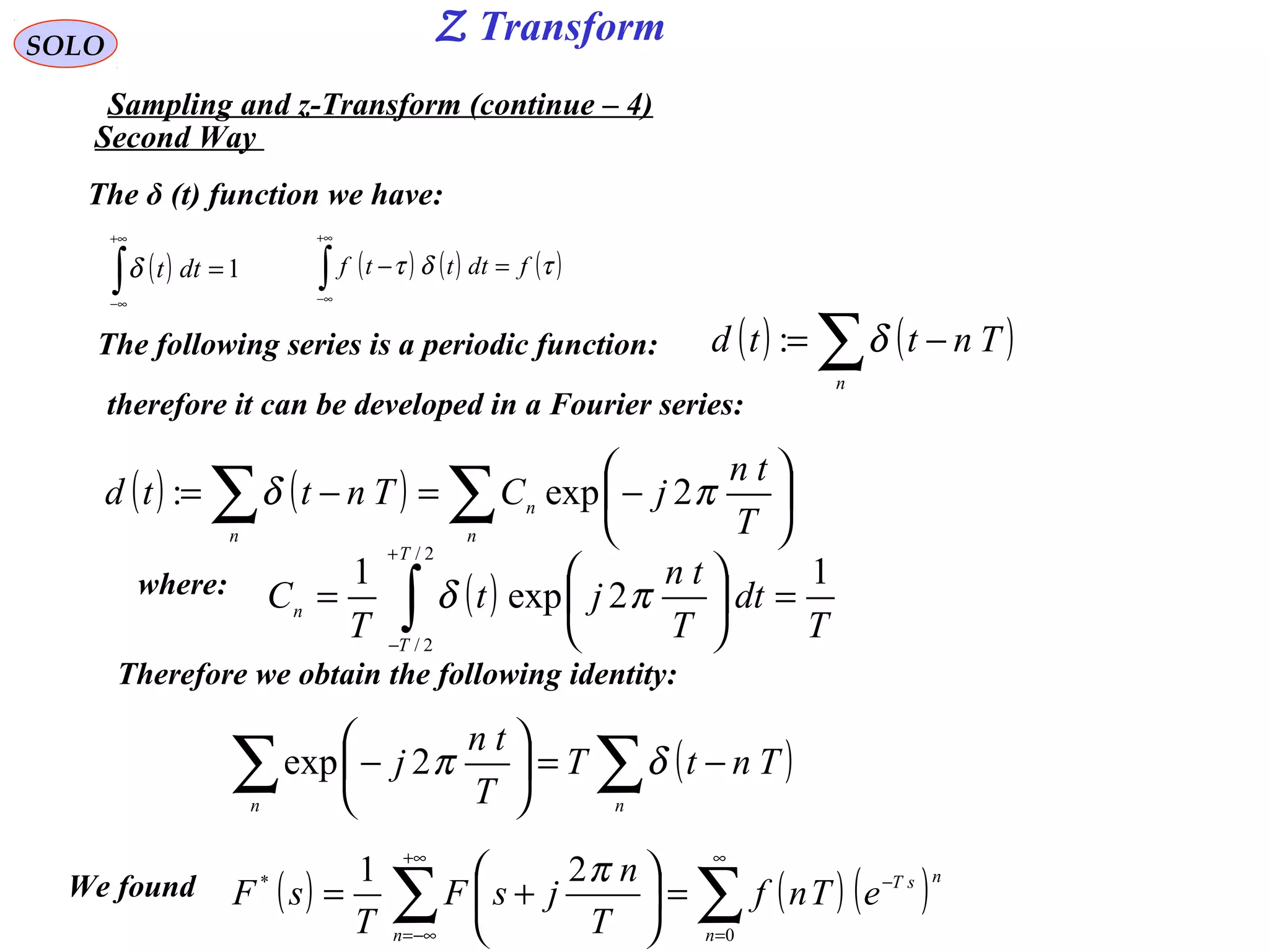
Sampling and z-Transform (continue – 5)
We found
Using the definition of the Fourier Transform and it’s inverse:
we obtain ( ) ( ) ( )∫
+∞
∞−
= ννπνπ dTnjFTnf 2exp2
( ) ( ) ( ) ( ) ( ) ( )∑∫∑
∞
=
+∞
∞−
∞
=
−=−=
0
111
0
*
exp2exp2exp
nn
n
sTndTnjFsTTnfsF ννπνπ
( ) ( ) ( )[ ]∫ ∑
+∞
∞−
+∞
−∞=
−−== 111
*
2exp22 νννπνπνπ dTnjFjsF
n
( ) ( ) ∑∫ ∑
+∞
−∞=
+∞
∞−
+∞
−∞=
−=
−−==
nn T
n
F
T
d
T
n
T
FjsF νπνννδνπνπ 2
11
22 111
*
We recovered (with –n instead of n) ( ) ∑
+∞
−∞=
+=
n T
n
jsF
T
sF
π21*
Second Way (continue)
Making use of the identity: with 1/T instead of T
and ν - ν 1 instead of t we obtain: ( )[ ] ∑∑
−−=−−
nn T
n
T
Tnj 11
1
2exp ννδννπ
( )∑∑ −=
−
nn
TntT
T
tn
j δπ2exp
Z Transform](https://image.slidesharecdn.com/complexvariables-140921180830-phpapp02/75/Mathematics-and-History-of-Complex-Variables-267-2048.jpg)
![Z TransformSOLO
Table of Z-Transform Functions
Z - Domain
k - Domain
( )kf ( ) ( ) f
k
k
RzzkfzF >= ∑
∞
=
−
0
1
( )mkf + ( ) ( ) ( ) ( )[ ]110 11
−−−−− +−−
mfzfzfzFz mm
2
( )mkf − ( )zFz m−
3
( ) ( ) ( )kfkfkf −+=∆ 1: ( ) ( ) ( )01 fzzFz −−4
( ) ( ) ( ) ( )kfkfkfkf ++−+=∆ 122:2
( ) ( ) ( ) ( ) ( )1021
2
fzfzzzFz −−−−5
( )kf3
∆ ( ) ( ) ( ) ( ) ( ) ( ) ( )2130331 23
fzfzzfzzzzFz −−−+−−−6](https://image.slidesharecdn.com/complexvariables-140921180830-phpapp02/75/Mathematics-and-History-of-Complex-Variables-271-2048.jpg)
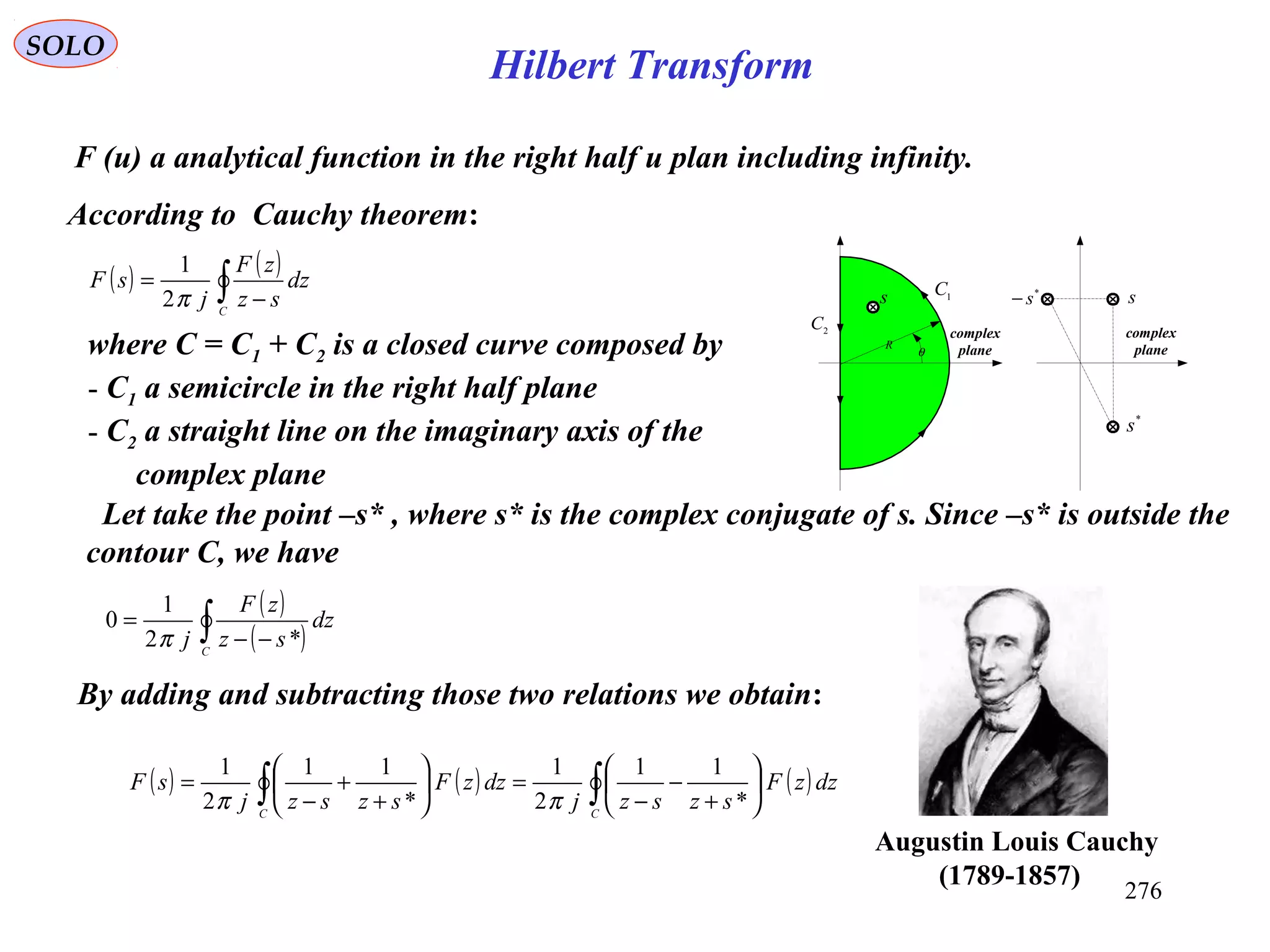
![277
SOLO
Let compute the integrals:
s
R
θ
1C
2C
s
*
s
*
s−
complex
plane
complex
plane
along C1, assuming R → ∞ we have
( )θjRszsz exp
1
*
11
≈
+
≈
−
( ) ( ) ( )∫∫
+
−
−
=
+
+
−
=
CC
dzzF
szszj
dzzF
szszj
sF
*
11
2
1
*
11
2
1
ππ
( ) θθ djRjzd exp=
( ) ( )[ ] ( ) 0exp2
2
1
lim
*
11
2
1
2
2
1
1
∞
−
→∞
=∞==
+
+
−
= ∫∫
atanalyticF
R
C
FdjRFj
j
dzzF
szszj
I
π
π
θθ
ππ
( ) 0
*
11
2
1
1
3 =
+
−
−
= ∫C
dzzF
szszj
I
π
along C2, assuming R → ∞ we have
( )
( )( )
( ) ( )
( )
( )∫∫∫
∞
∞−
=
−=
+=
∞
∞−
−+
−
=
+−
+−
=
+
+
−
=
j
j
vjz
js
js
j
jC
vdvjF
v
vj
zdzF
szsz
ssz
j
dzzF
szszj
I 22
*
2
1
*
*2
2
1
*
11
2
1
2
ωσ
ω
πππ ωσ
ωσ
( )
( )( )
( )
( )
( )∫∫∫
∞
∞−
=
−=
+=
∞
∞−
−+
=
+−
+
=
+
−
−
=
j
j
vjz
js
js
j
jC
vdvjF
v
dzzF
szsz
ss
j
dzzF
szszj
I 22
*
4
1
*
*
2
1
*
11
2
1
2
ωσ
σ
πππ ωσ
ωσ
( ) ( )
( )
( )
( )
( )∫∫
∞
∞−
∞
∞−
−+
=
−+
−
=
j
j
j
j
vdvjF
v
vdvjF
v
vj
sF 2222
11
ωσ
σ
πωσ
ω
π
Hilbert Transform](https://image.slidesharecdn.com/complexvariables-140921180830-phpapp02/75/Mathematics-and-History-of-Complex-Variables-277-2048.jpg)
![278
SOLO
Let write
( ) ( )
( )
( ) ( )
( )
( )∫∫
∞
∞−
∞
∞−
−+
=∞+
−+
−
=
j
j
j
j
vdvjF
v
FvdvjF
v
vj
sF 2222
11
ωσ
σ
πωσ
ω
π
( ) ( )[ ] ( )[ ]ωσωσωσ jFjjFjF +++=+ ImRe
( ){ } ( )[ ] ( )
( )
( )[ ] ( )[ ]( )
( )
( )[ ] ( )[ ]( )∫
∫
∞
∞−
∞
∞−
+
−+
=
+
−+
−
=+++
j
j
j
j
vdjFjjF
v
vdjFjjF
v
vj
jFjjF
νν
ωσ
σ
π
νν
ωσ
ω
π
ωσωσ
ImRe
1
ImRe
1
ImRe
22
22
We obtain
By equaling the real and imaginary parts we obtain
( )[ ] ( )
( )
( )[ ]
( )
( )[ ]∫∫
∞
∞−
∞
∞−
−+
=
−+
−
=+
j
j
j
j
vdvjF
v
vdvjF
v
v
jF Re
1
Im
1
Re 2222
ωσ
σ
πωσ
ω
π
ωσ
( )[ ] ( )
( )
( )[ ]
( )
( )[ ]∫∫
∞
∞−
∞
∞−
−+
=
−+
−
=+
j
j
j
j
vdvjF
v
vdvjF
v
v
jF Im
1
Re
1
Im 2222
ωσ
σ
πωσ
ω
π
ωσ
From those relation we can see that if F (s) is analytic in the right half plane,
then it is enough to know it’s value on the imaginary axis to compute F (s) in
the entire right half plane.
Hilbert Transform](https://image.slidesharecdn.com/complexvariables-140921180830-phpapp02/75/Mathematics-and-History-of-Complex-Variables-278-2048.jpg)
![279
SOLO
We are interested in cases when σ = 0, i.e. points on the imaginary axis. In this
case:
( )[ ] ( )
( )
( )[ ]
( )
( )[ ]∫∫
∞
∞−
∞
∞−
−+
=
−+
−
=+
j
j
j
j
vdvjF
v
vdvjF
v
v
jF Re
1
Im
1
Re 2222
ωσ
σ
πωσ
ω
π
ωσ
( )[ ] ( )
( )
( )[ ]
( )
( )[ ]∫∫
∞
∞−
∞
∞−
−+
=
−+
−
=+
j
j
j
j
vdvjF
v
vdvjF
v
v
jF Im
1
Re
1
Im 2222
ωσ
σ
πωσ
ω
π
ωσ
It seams that we have a singular point ν = ω, on the path of integration, but we
will see how this can be taken care.
( )[ ] ( )[ ]
( )∫
∞
∞−
−
=
j
j
vd
v
vjF
jF
ωπ
ω
Im1
Re
( )[ ] ( )[ ]
( )∫
∞
∞−
−
=
j
j
vd
v
vjF
jF
ωπ
ω
Re1
Im
Hilbert Transform](https://image.slidesharecdn.com/complexvariables-140921180830-phpapp02/75/Mathematics-and-History-of-Complex-Variables-279-2048.jpg)
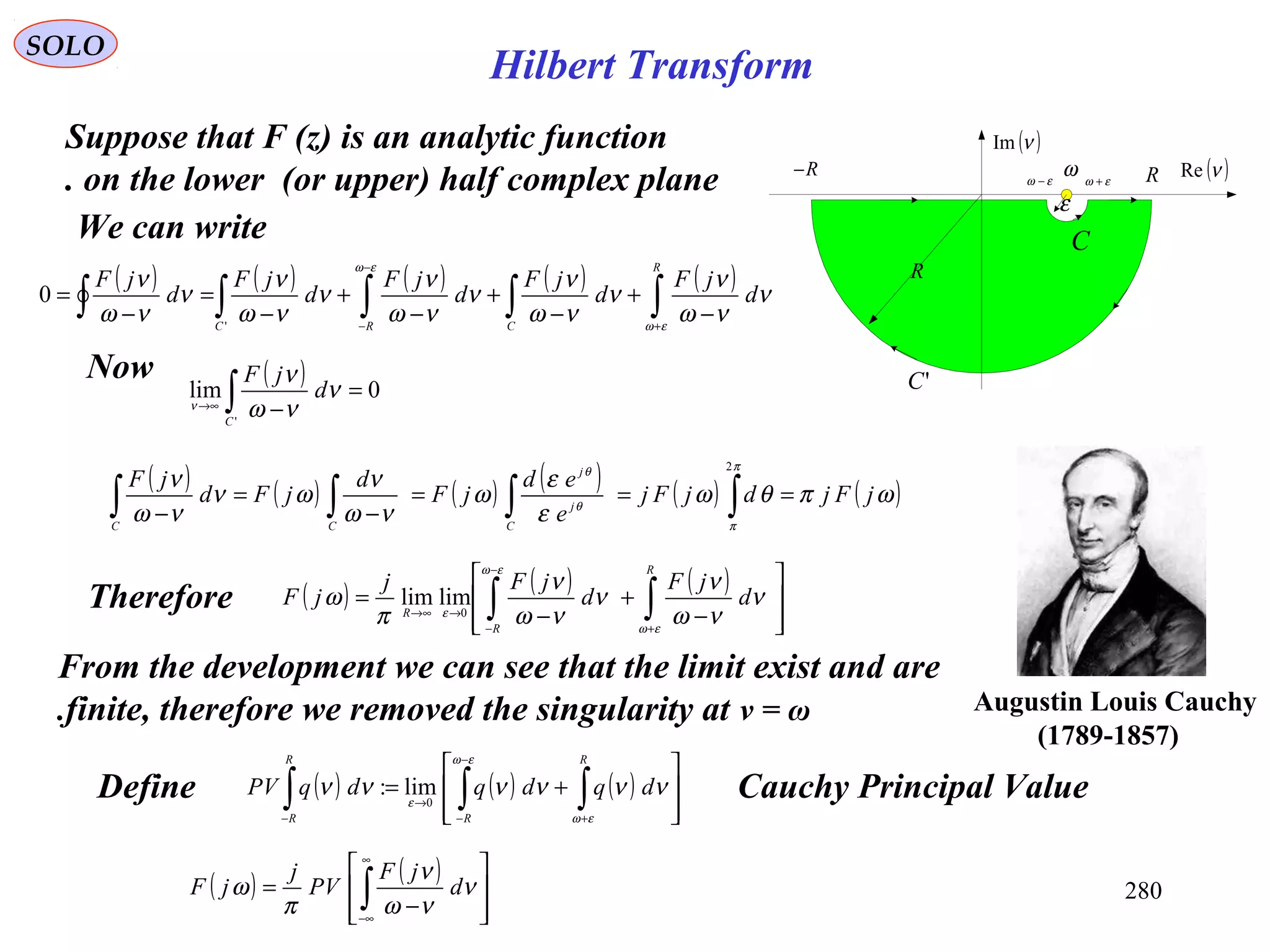
![281
SOLO
Suppose that F (z) is an analytic function
on the lower (or upper) half complex plane.
We can write
( ) ( )[ ] ( )[ ] ( )[ ] ( )[ ]
−
+
−
−=+= ∫∫
∞
∞−
∞
∞−
ν
νωπ
ν
νωπ
ωωω d
vjF
PV
j
d
vjF
PVjFjjFjF
ReIm1
ImRe
Comparing real and imaginary parts we obtain
( )[ ] ( )[ ] ( )[ ]{ }
( )[ ] ( )[ ] ( )[ ]{ }ων
νωπ
ω
ων
νωπ
ω
jFd
vjF
PVjF
jFd
vjF
PVjF
Re
Re1
Im
Im
Im1
Re
H
H
=
−
=
−=
−
−=
∫
∫
∞
∞−
∞
∞−
Where H stands for Hilbert Transform.
( ) ( )
−
= ∫
∞
∞−
ν
νω
ν
π
ω d
jF
PV
j
jF
( )νRe
( )νIm
ω εω +εω −
R
RR−
'C
C
ε
David Hilbert
1862 - 1943
Return to Table of Contents
Hilbert Transform](https://image.slidesharecdn.com/complexvariables-140921180830-phpapp02/75/Mathematics-and-History-of-Complex-Variables-281-2048.jpg)
![282
SOLO
References
[2] Churchill, R.V., “Complex Variables and Applications”, McGraw-Hill, Kõgakusha’
1960
[3] Spiegel, M.R., “Complex Variables with an introduction to Conformal Mapping
and its applications”, Schaum’s Outline Series, McGraw-Hill, 1964
[4] Hauser, A.A., “Complex Variables with Physical Applications”, Simon & Schuster,
1971
[5] Fisher, S.D., “Complex Variables”, Wadsworth & Brooks/Cole Mathematics Series,
1986
Complex Variables
[6] Tristan, N., “Visual Complex Analysis”, Clarendon Press, Oxford, 1997
[1] E.C. Titchmarsh, “The Theory of Functions”, Oxford University Press, 2nd
Ed., 1939
http://www.ima.umn.edu/~arnold/complex.html](https://image.slidesharecdn.com/complexvariables-140921180830-phpapp02/75/Mathematics-and-History-of-Complex-Variables-282-2048.jpg)


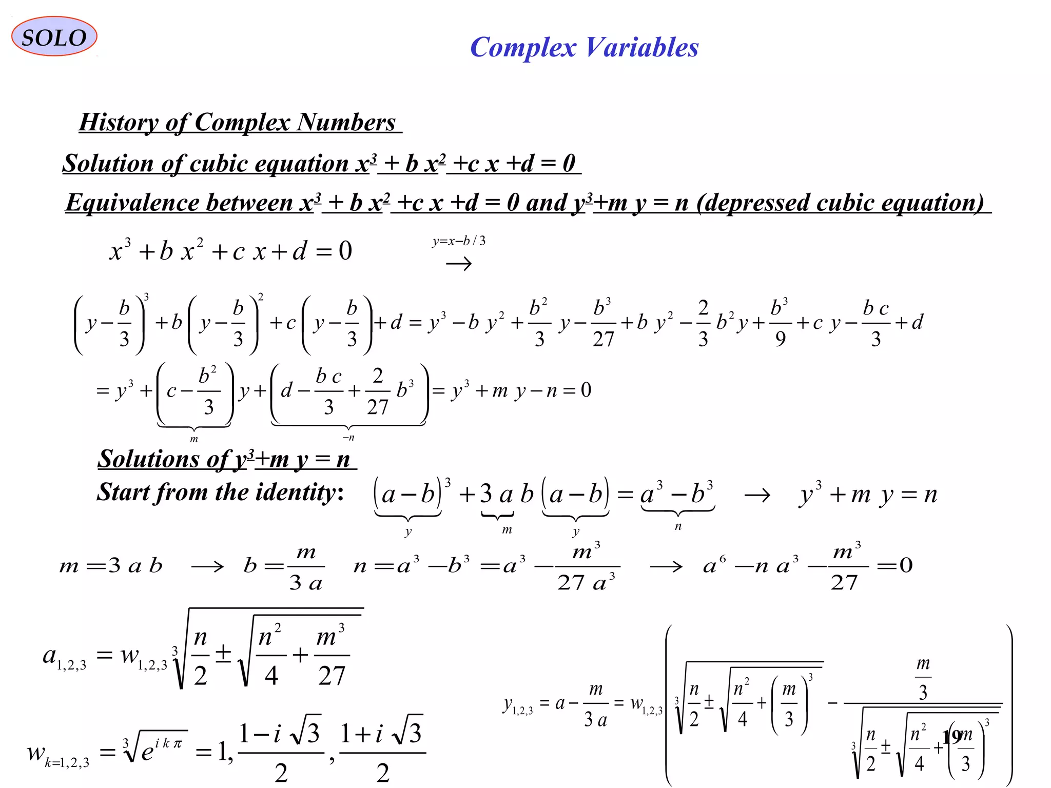
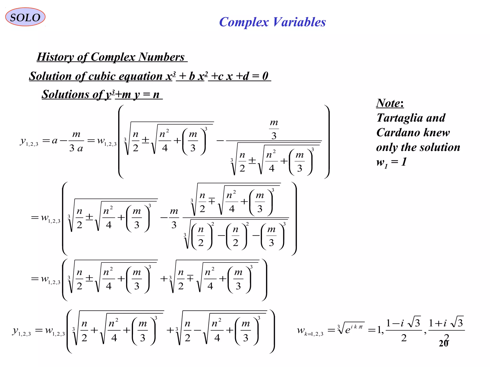
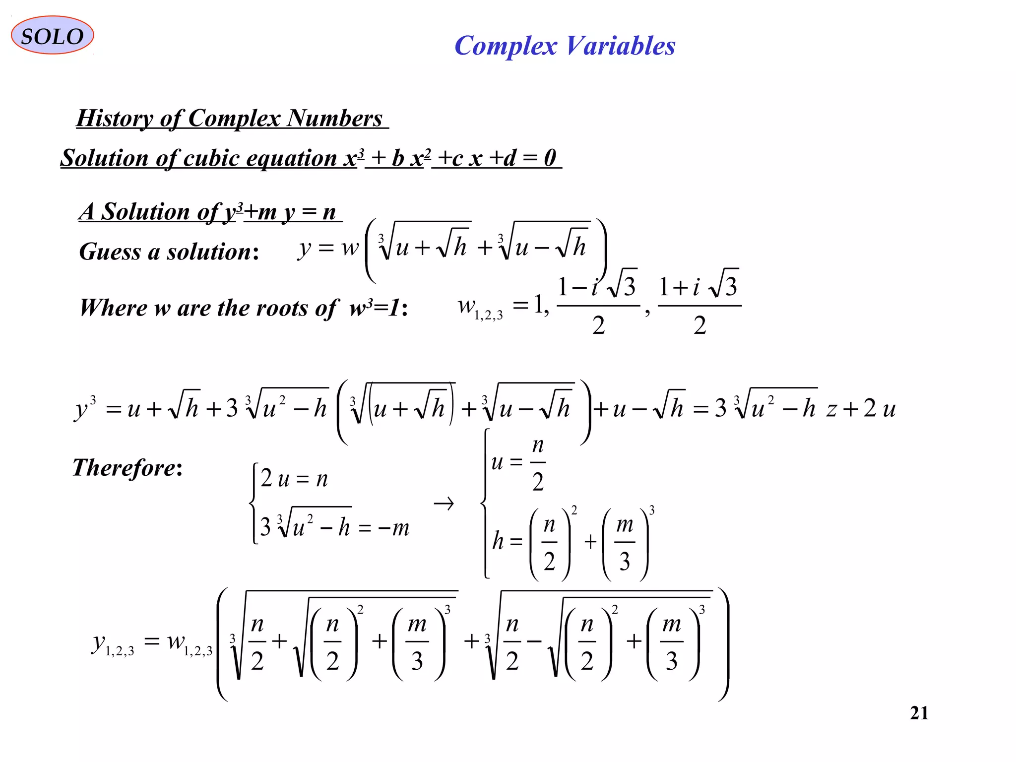
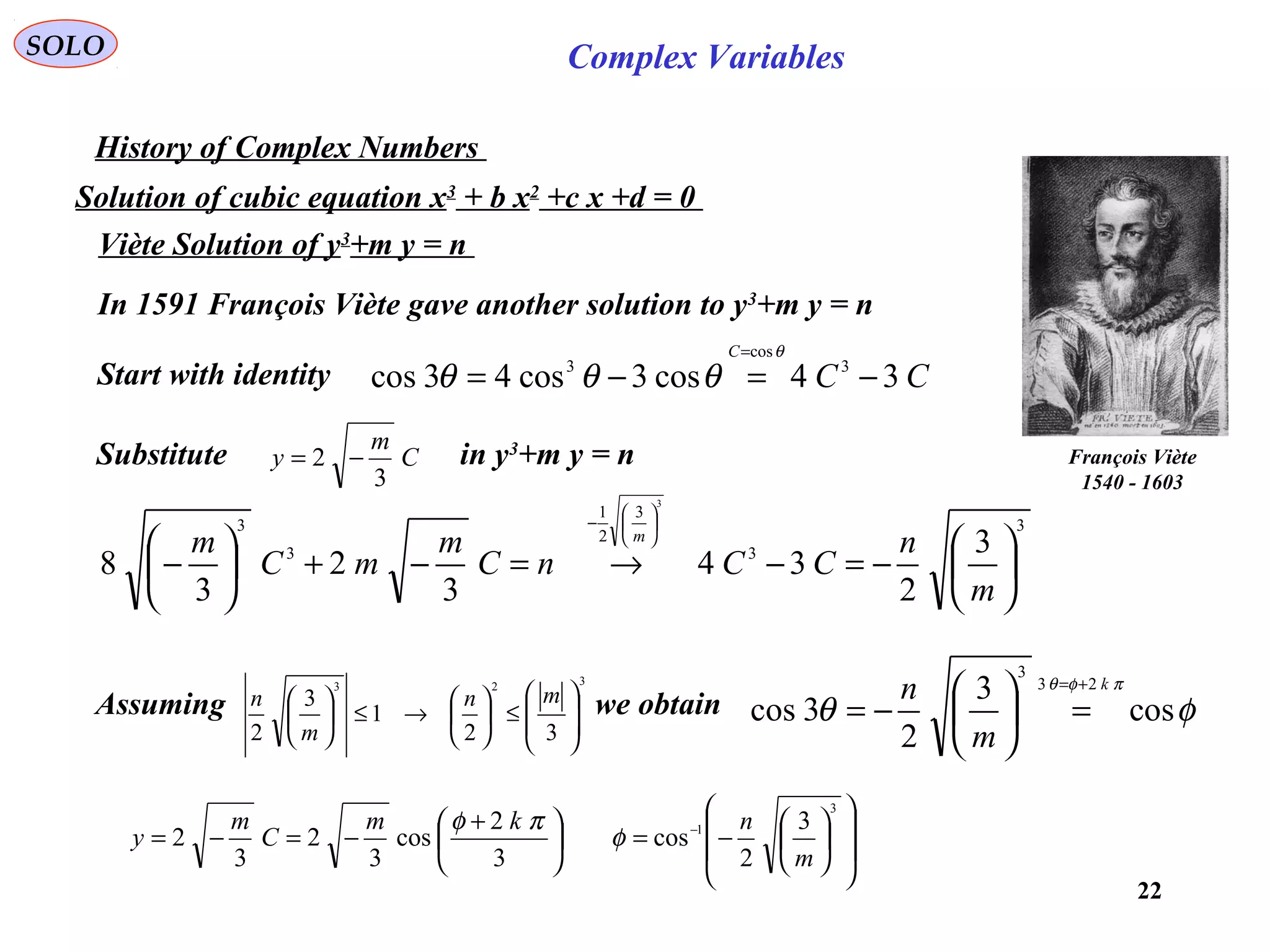
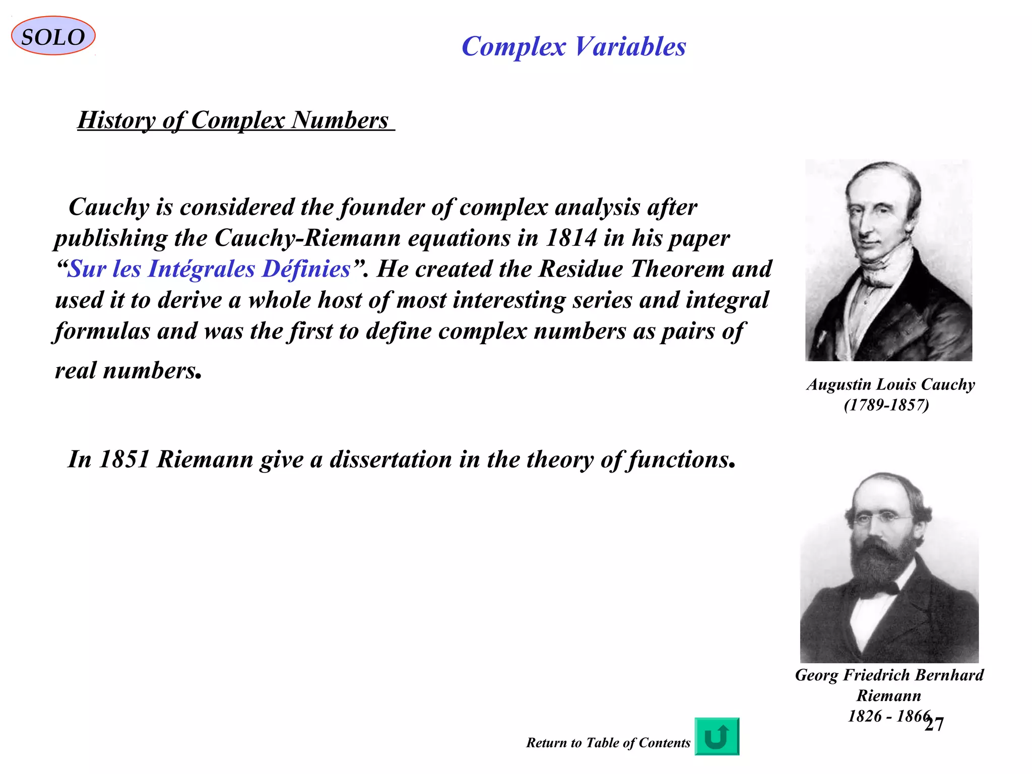
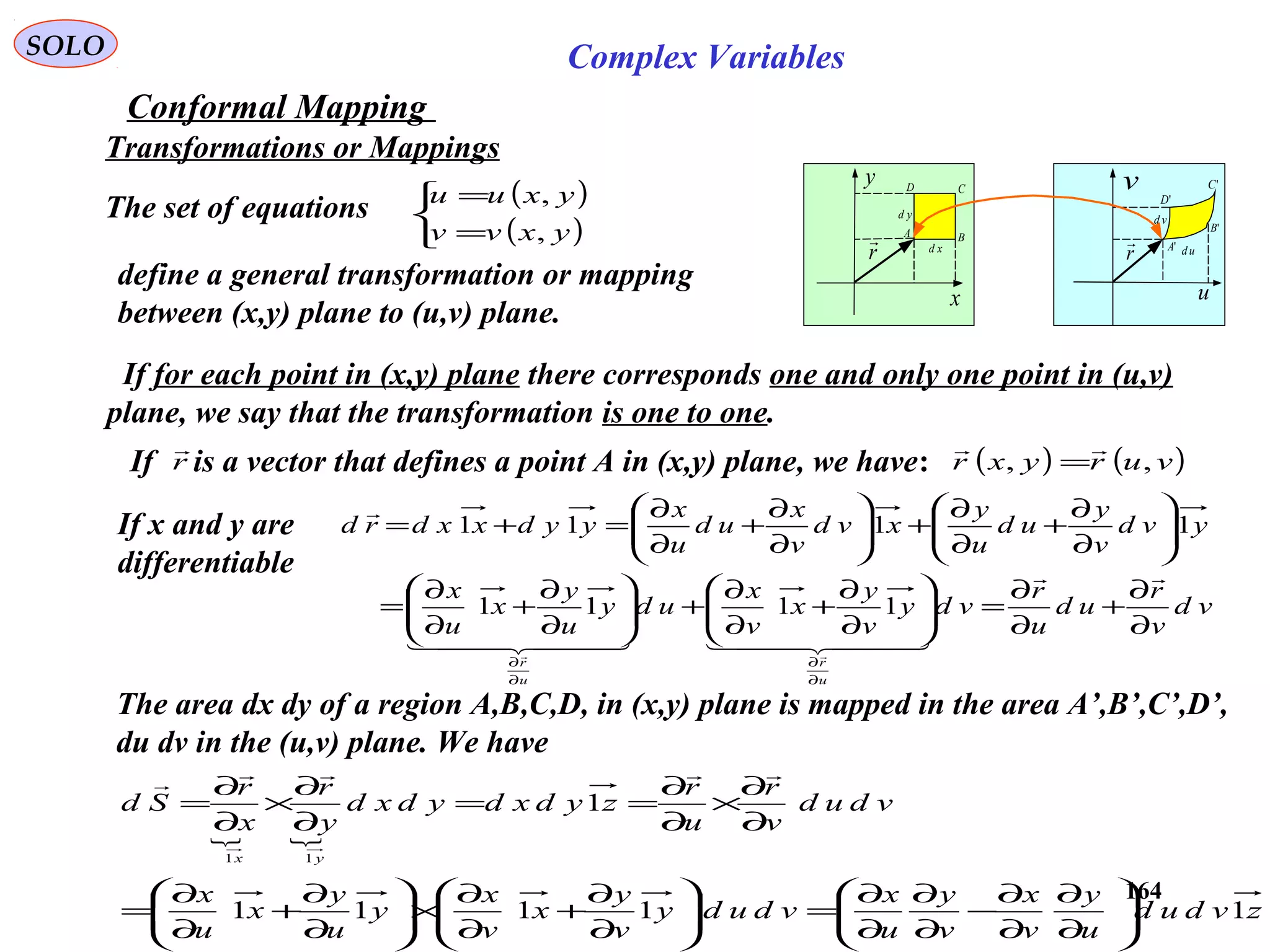
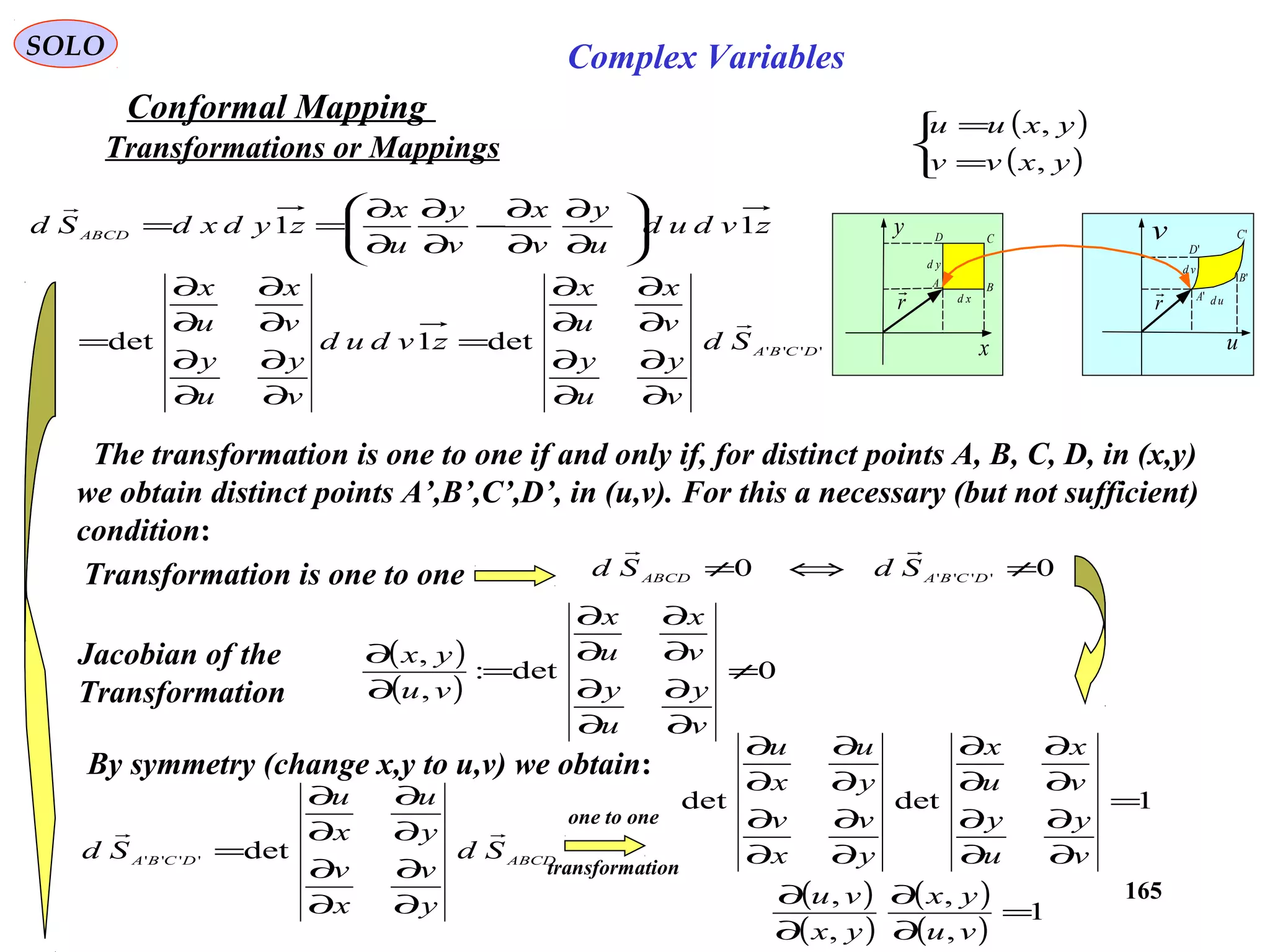
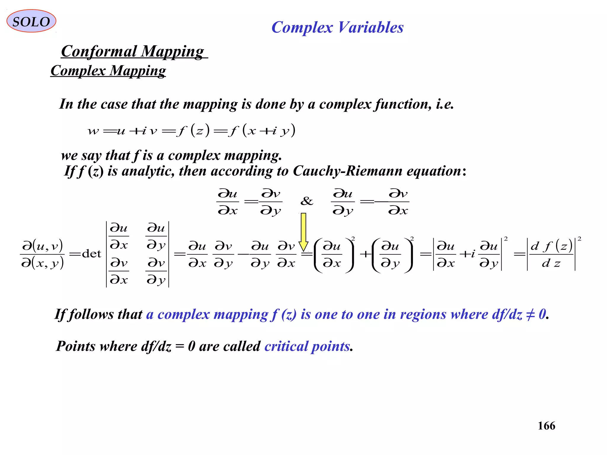
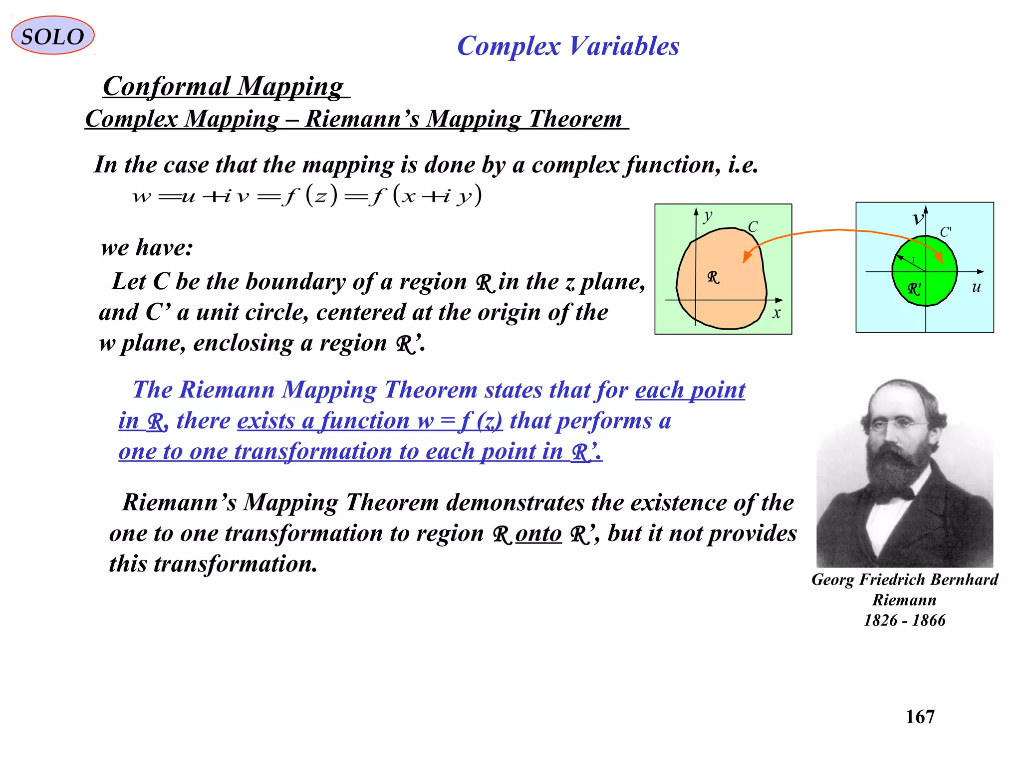
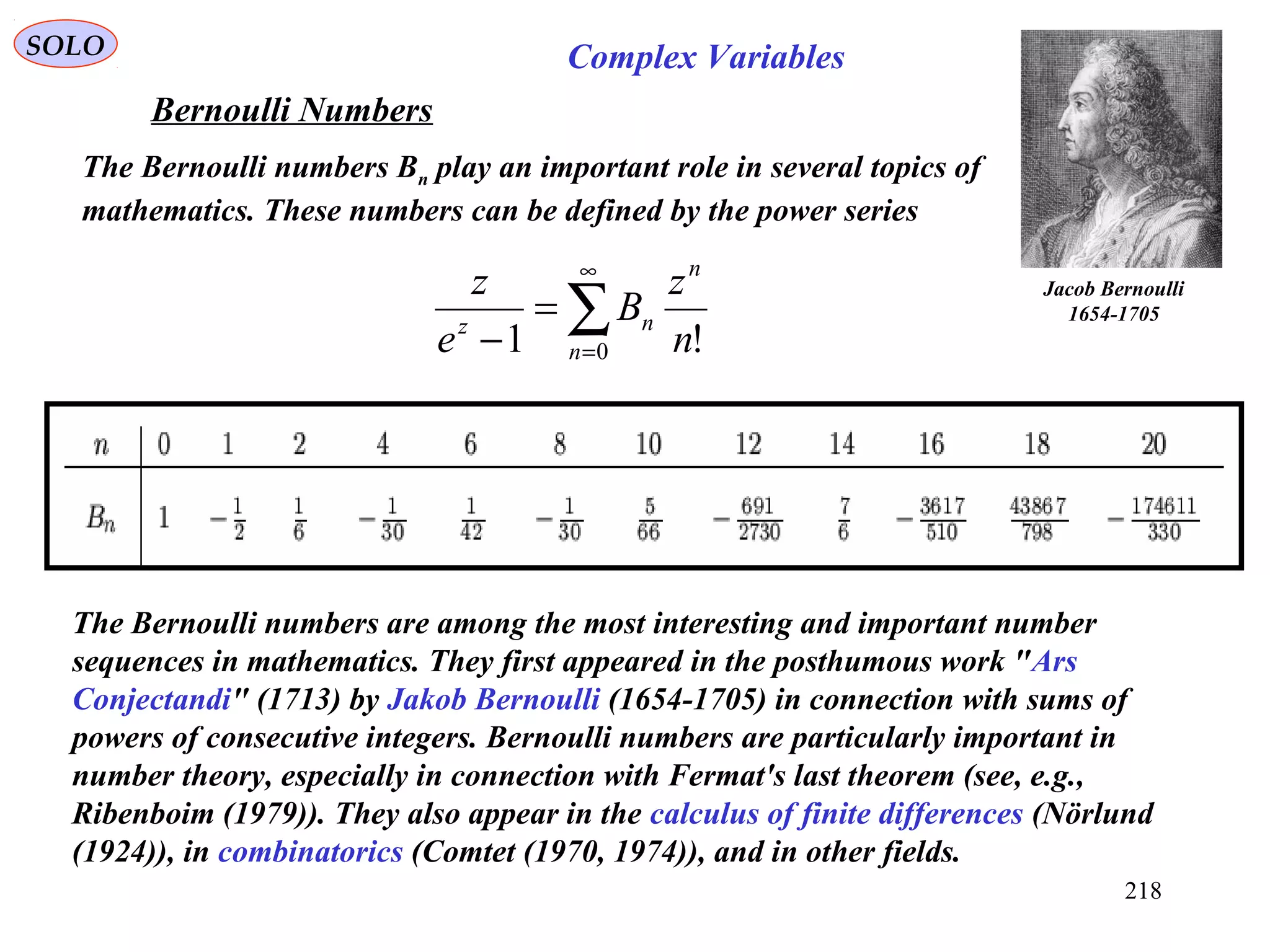
The document is a comprehensive overview of complex variables, covering fundamental definitions, operations, and the historical development of complex numbers. It includes detailed discussions on the axiomatic foundations, significant theorems, and key figures in the history of complex analysis. The document serves as a resource for understanding complex number systems, their properties, and their applications.