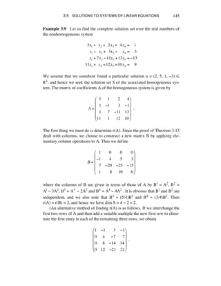
This document introduces matrices through the theory of simultaneous linear equations. It discusses how matrices can represent systems of linear equations and how elementary row operations can be used to solve such systems. Specifically, it shows that elementary row operations preserve equivalence between systems of linear equations. It then provides examples of using row operations to determine that a system has no solution and to solve a system with an infinite number of solutions.


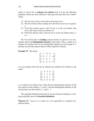
![LINEAR EQUATIONS AND MATRICES126
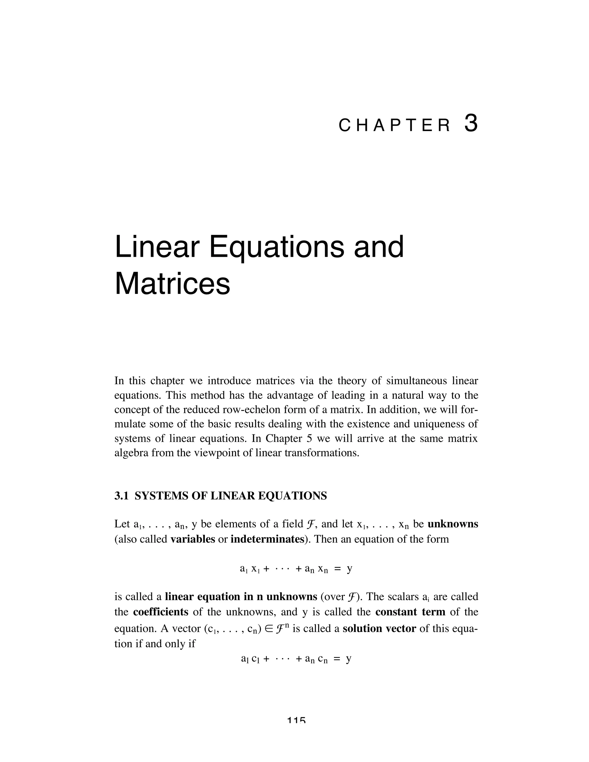
(a)!!
1 !2 !3 !1
2 !1 !2 !!2
3 !!1 !2 !!3
"
#
$
$
$
%
&
'
'
'
!!!!!!!!!!!!!!!!!!!(b)!!
1 !2 !1 !!2 !1
2 !4 !!1 !2 !3
3 !6 !!2 !6 !5
"
#
$
$
$
%
&
'
'
'
(c)!!
1 !3 !1 !2
0 !1 !5 !3
2 !5 !!3 !1
4 !1 !!1 !5
"
#
$
$
$
$
%
&
'
'
'
'
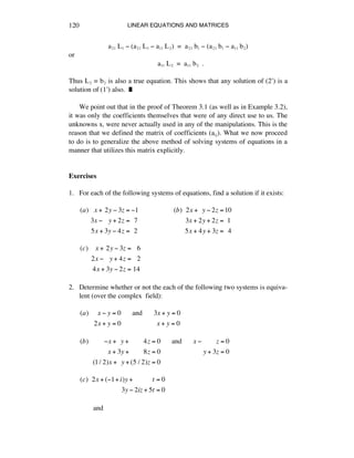
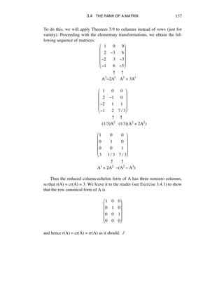
3. For each of the following systems, find a solution or show that no solution
exists:
(a)!!!!!x +!!y +!!!z =1
2x ! 3y + 7z = 0
!!3x ! 2y + 8z = 4
(b)!!!!!x ! y + 2z =1
x +!y +!!z = 2
2x !!y +!!z = 5
(c)!!!!!x ! y + 2z = 4
3x + y + 4z = 6
x + y +!!!z =1
(d)!!!!!x + 3y +!!!z = 2
2x + 7y + 4z = 6
x +!!y ! 4z =1
(e)!!!!!x +!3y +!!!z = 0
2x + 7y + 4z = 0
x +!!!y ! 4z = 0
( f )!!!!2x !!!y + 5z =19
x + 5y ! 3z = 4
3x + 2y + 4z = 5
(g)!!!!2x !!!y + 5z =19
x + 5y ! 3z = 4
3x + 2y + 4z = 25
4. Let fè, fì and f3 be elements of F[®] (i.e., the space of all real-valued func-
tions defined on ®).
(a) Given a set {xè, xì, x3} of real numbers, define the 3 x 3 matrix F(x) =
(fá(xé)) where the rows are labelled by i and the columns are labelled by j.
Prove that the set {fá} is linearly independent if the rows of the matrix F(x)
are linearly independent.
(b) Now assume that each fá has first and second derivatives defined on
some interval (a, b) ™ ®, and let fá(j) denote the jth derivative of fá (where
fá(0) is just fá). Define the matrix W(x) = (fá(j-1 )(x)) where 1 ¯ i, j ¯ 3.
Prove that {fá} is linearly independent if the rows of W(x) are independent](https://image.slidesharecdn.com/07chap3-150213074831-conversion-gate01/85/07-chap3-12-320.jpg)
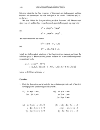
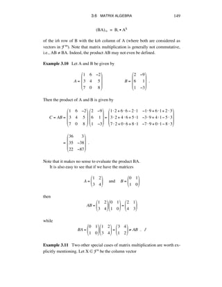
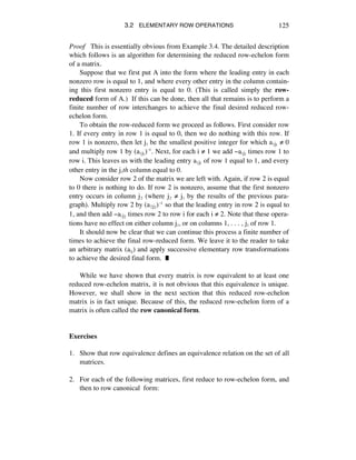
![3.6 MATRIX ALGEBRA 151
X =
x1
!
xn
!
"
#
#
#
$
%
&
&
&
' Fn and Y =
y1
!
ym
!
"
#
#
#
$
%
&
&
&
' Fm .
If we consider X to be an n x 1 matrix and Y to be an m x 1 matrix, then we
may write this system in matrix notation as
AX = Y .
Note that the ith row vector of A is Aá = (aáè, . . . , aáñ) so that the expression
Íéaáéxé = yá may be written as the standard scalar product
Aá Â X = yá .
We leave it to the reader to show that if A is an n x n matrix, then
A Iñ = IñA = A .
Even if A and B are both square matrices (i.e., matrices of the form m x m),
the product AB will not generally be the same as BA unless A and B are
diagonal matrices (see Exercise 3.6.4). However, we do have the following.
Theorem 3.17 For matrices of proper size (so that these operations are
defined), we have:
(a) (AB)C = A(BC) (associative law).
(b) A(B + C) = AB + AC (left distributive law).
(c) (B + C)A = BA + CA (right distributive law).
(d) k(AB) = (kA)B = A(kB) for any scalar k.
Proof (a)!![(AB)C]ij = !k (AB)ik ckj = !r,!k (airbrk )ckj = !r,!kair (brkckj )
= !rair (BC)rj = [A(BC)]ij !!.
(b)!![A(B + C)]ij = !kaik (B + C)kj = !kaik (bkj + ckj )
= !kaikbkj + !kaikckj = (AB)ij + (AC)ij
= [(AB)+ (AC)]ij !!.
(c) Left to the reader (Exercise 3.6.1).
(d) Left to the reader (Exercise 3.6.1). ˙](https://image.slidesharecdn.com/07chap3-150213074831-conversion-gate01/85/07-chap3-37-320.jpg)
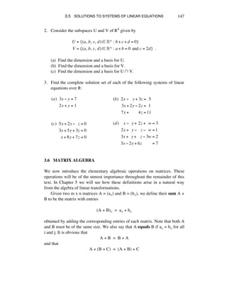
![LINEAR EQUATIONS AND MATRICES152
Given a matrix A = (aáé), we define the transpose of A, denoted by AT =
(aTij) to be the matrix with entries given by aTáé = aéá. In other words, if A is an
m x n matrix, then AT is an n x m matrix whose columns are just the rows of
A. Note in particular that a column vector is just the transpose of a row vector.
Example 3.12 If A is given by
!
1 2 3
4 5 6
!
"
#
$
%
&
then AT is given by
!
1 4
2 5
3 6
!
"
#
#
#
$
%
&
&
&
!!. ∆
Theorem 3.18 The transpose has the following properties:
(a) (A + B)T = AT + BT.
(b) (AT)T = A.
(c) (cA)T = cAT for any scalar c.
(d) (AB)T = BT AT.
Proof (a) [(A + B)T]áé = [(A + B)]éá = aéá + béá = aTáé + bTáé = (AT + BT)áé.
(b) (AT)Táé = (AT)éá = aáé = (A)áé.
(c) (cA)Táé = (cA)éá = caéá = c(AT)áé.
(d) (AB)Táé = (AB)éá = Ík aéÉbÉá = Ík bTáÉaTÉé = (BT AT)áé. ˙
We now wish to relate this algebra to our previous results dealing with the
rank of a matrix. Before doing so, let us first make some elementary observa-
tions dealing with the rows and columns of a matrix product. Assume that
A ∞ Mmxn(F) and B ∞ Mnxr(F) so that the product AB is defined. Since the
(i, j)th entry of AB is given by (AB)áé = ÍÉaáÉbÉé, we see that the ith row of AB
is given by a linear combination of the rows of B:
(AB)á = (ÍÉaáÉbÉè, . . . , ÍÉaáÉbkr) = ÍÉaáÉ(bÉè, . . . , bkr) = ÍkaáÉBÉ .
Another way to write this is to observe that](https://image.slidesharecdn.com/07chap3-150213074831-conversion-gate01/85/07-chap3-38-320.jpg)
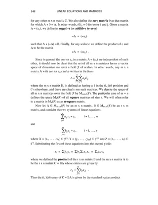
![LINEAR EQUATIONS AND MATRICES154
while
r(AB) = dim WAB ¯ dim WA = r(A) . ˙
Exercises
1. Complete the proof of Theorem 3.17.
2. Prove Theorem 3.19.
3. Let A be any m x n matrix and let X be any n x 1 matrix, both with
entries in F. Define the mapping f : Fn ‘Fm by f(X) = AX.
(a) Show that f is a linear transformation (i.e., a vector space homomor-
phism).
(b) Define Im f = {AX: X ∞ Fn}. Show that Im f is a subspace of Fm.
(c) Let U be the column space of A. Show that Im f = U. [Hint: Use
Example 3.11 to show that Im f ™ U. Next use the equation (AI)j = AIj to
show that U ™ Im f.]
(d) Let N denote the solution space to the system AX = 0. In other
words, N = {X ∞ Fn: AX = 0}. (N is usually called the null space of A.)
Show that
dim N + dim U = n .
[Hint: Suppose dim N = r, and extend a basis {xè, . . . , xr} for N to a
basis {xá} for Fn. Show that U is spanned by the vectors Axr+1 , . . . ,
Axn , and then that these vectors are linearly independent. Note that this
exercise is really just another proof of Theorem 3.13.]
4. A matrix of the form
a11 0 0 ! 0
0 a22 0 ! 0
" " " "
0 0 0 ! ann
!
"
#
#
#
#
$
%
&
&
&
&
is called a diagonal matrix. In other words, A = (aáé) is diagonal if aáé = 0
for i ≠ j. If A and B are both square matrices, we may define the commu-
tator [A, B] of A and B to be the matrix [A, B] = AB - BA. If [A, B] = 0,
we say that A and B commute.
(a) Show that any diagonal matrices A and B commute.](https://image.slidesharecdn.com/07chap3-150213074831-conversion-gate01/85/07-chap3-40-320.jpg)
![3.6 MATRIX ALGEBRA 155
(b) Prove that the only n x n matrices which commute with every n x n
diagonal matrix are diagonal matrices.
5. Given the matrices
6.
A =!
!!2 !1
!!1 !!0
!3 !!4
"
#
$
$
$
%
&
'
'
'
!!!!!!!!!!B =!
1 !2 !5
3 !!4 !!0
"
#
$
%
&
'
compute the following:
(a) AB.
(b) BA.
(c) AAT.
(d) ATA.
(e) Verify that (AB)T = BTAT.
6. Consider the matrix A ∞ Mn(F) given by
A =!
0 1 0 0 ! 0 0
0 0 1 0 ! 0 0
0 0 0 1 ! 0 0
" " " " " "
0 0 0 0 ! 0 1
0 0 0 0 ! 0 0
!
"
#
#
#
#
#
#
#
$
%
&
&
&
&
&
&
&
!!.
Thus A has zero entries everywhere except on the superdiagonal where
the entries are 1’s. Let A2 = AA, A3 = AAA, and so on. Show that An = 0
but An-1 ≠ 0.
7. Given a matrix A = (aáé) ∞ Mn(F), the sum of the diagonal elements of A
is called the trace of A, and is denoted by Tr A. Thus
Tr A = aii !!.
i=1
n
!
(a) Prove that Tr(A + B) = Tr A + Tr B and that Tr(åA) = å(Tr A) for
any scalar å.
(b) Prove that Tr(AB) = Tr(BA).
8. (a) Prove that it is impossible to find matrices A, B ∞ Mn(®) such that
their commutator [A, B] = AB - BA is equal to 1.](https://image.slidesharecdn.com/07chap3-150213074831-conversion-gate01/85/07-chap3-41-320.jpg)
![LINEAR EQUATIONS AND MATRICES156
(b) Let F be a field of characteristic 2 (i.e., a field in which 1 + 1 = 0; see
Exercise 1.5.17). Prove that it is possible to find matrices A, B ∞ M2(F)
such that [A, B] = 1.
9. A matrix A = (aáé) is said to be upper-triangular if aáé = 0 for i > j. In
other words, every entry of A below the main diagonal is zero. Similarly,
A is said to be lower-triangular if aáé = 0 for i < j. Prove that the product
of upper (lower) triangular matrices is an upper (lower) triangular matrix.
10. Consider the so-called Pauli spin matrices
!1 =
0 1
1 0
"
#
$
%
&
'!!!!!!!!!!!2 =
0 (i
i 0
"
#
$
%
&
'!!!!!!!!!!!3 =
1 0
0 (1
"
#
$
%
&
'
and define the permutation symbol ´ijk by
!ijk =
!!1 !!if (i,! j,!k) is an even permutation of (1,!2,!3)
"1 !!!if (i,! j,!k) is an odd permutation of (1,!2,!3)
0 if any two indices are the same!!!!!!!!!!!!!!!!!!!
!!.
#
$
%
&
%
The commutator of two matrices A, B ∞ Mn(F) is defined by [A, B] =
AB - BA, and the anticommutator is given by [A, B]+ = AB + BA.
(a) Show that [ßá, ßé] = 2i ÍÉ´ijk ßÉ. In other words, show that ßáßé = ißÉ
where (i, j, k) is an even permutation of (1, 2, 3).
(b) Show that [ßá, ßé]+ = 2I∂áé .
(c) Using part (a), show that Tr ßá = 0.
(d) For notational simplicity, define ßà = I. Show that {ß0, ß1, ß2, ß3}
forms a basis for M2(ç). [Hint: Show that Tr(ßå ß∫) = 2∂å∫ where 0 ¯ å,
∫ ¯ 3. Use this to show that {ßå} is linearly independent.]
(e) According to part (d), any X ∞ M2(ç) may be written in the form X =
Íåxåßå. How would you find the coefficients xå?
(f) Show that Óßå, ß∫Ô = (1/2)Tr(ßåß∫) defines an inner product on
M2(ç).
(g) Show that any matrix X ∞ M2(ç) that commutes with all of the ßá
(i.e., [X, ßá] = 0 for each i = 1, 2, 3) must be a multiple of the identity
matrix.](https://image.slidesharecdn.com/07chap3-150213074831-conversion-gate01/85/07-chap3-42-320.jpg)
![3.6 MATRIX ALGEBRA 157
11. A square matrix S is said to be symmetric if ST = S, and a square matrix
A is said to be skewsymmetric (or antisymmetric) if AT = -A. (We
continue to assume as usual that F is not of characteristic 2.)
(a) Show that S ≠ 0 and A are linearly independent in Mn(F).
(b) What is the dimension of the space of all n x n symmetric matrices?
(c) What is the dimension of the space of all n x n antisymmetric
matrices?
12. Find a basis {Aá} for the space Mn(F) that consists only of matrices with
the property that Aá2 = Aá (such matrices are called idempotent or
projections). [Hint: The matrices
1 0
0 0
!
"
#
$
%
&!!!!!!
1 1
0 0
!
"
#
$
%
&!!!!!!
0 0
1 0
!
"
#
$
%
&!!!!!!
0 0
1 1
!
"
#
$
%
&
will work in the particular case of M2(F).]
13. Show that it is impossible to find a basis for Mn(F) such that every pair
of matrices in the basis commute with each other.
14. (a) Show that the set of all nonsingular n x n matrices forms a spanning
set for Mn(F). Exhibit a basis of such matrices.
(b) Repeat part (a) with the set of all singular matrices.
15. Show that the set of all matrices of the form AB - BA do not span
Mn(F). [Hint: Use the trace.]
16. Is it possible to span Mn(F) using powers of a single matrix A? In other
words, can {Iñ , A, A2, . . . , An, . . .} span Mn(F)? [Hint: Consider
Exercise 4 above.]
3.7 INVERTIBLE MATRICES
We say that a matrix A ∞ Mñ(F) is nonsingular if r(A) = n, and singular if
r(A) < n. Given a matrix A ∞ Mñ(F), if there exists a matrix B ∞ Mñ(F) such
that AB = BA = Iñ, then B is called an inverse of A, and A is said to be
invertible.
Technically, a matrix B is called a left inverse of A if BA = I, and a
matrix Bæ is a right inverse of A if ABæ = I. Then, if AB = BA = I, we say that
B is a two-sided inverse of A, and A is then said to be invertible.](https://image.slidesharecdn.com/07chap3-150213074831-conversion-gate01/85/07-chap3-43-320.jpg)
![3.7 INVERTIBLE MATRICES 163
(b) Repeat part (a) where A is any m x n matrix and B is any n x m
matrix with n < m.
10. Summarize several of our results by proving the equivalence of the fol-
lowing statements for any n x n matrix A:
(a) A is invertible.
(b) The homogeneous system AX = 0 has only the zero solution.
(c) The system AX = Y has a solution X for every n x 1 matrix Y.
11. Let A and B be square matrices of size n, and assume that A is
nonsingular. Prove that r(AB) = r(B) = r(BA).
12. A matrix A is called a left zero divisor if there exists a nonzero matrix B
such that AB = 0, and A is called a right zero divisor if there exists a
nonzero matrix C such that CA = 0. If A is an m x n matrix, prove that:
(a) If m < n, then A is a left zero divisor.
(b) If m > n, then A is a right zero divisor.
(c) If m = n, then A is both a left and a right zero divisor if and only if A
is singular.
13. Let A and B be nonsingular symmetric matrices for which AB - BA = 0.
Show that AB, AîB, ABî and AîBî are all symmetric.
3.8 ELEMENTARY MATRICES
Recall the elementary row operations å, ∫, © described in Section 3.2. We now
let e denote any one of these three operations, and for any matrix A we define
e(A) to be the result of applying the operation e to the matrix A. In particular,
we define an elementary matrix to be any matrix of the form e(I). The great
utility of elementary matrices arises from the following theorem.
Theorem 3.22 If A is any m x n matrix and e is any elementary row opera-
tion, then
e(A) = e(Im)A .
Proof We must verify this equation for each of the three types of elementary
row operations. First consider an operation of type å. In particular, let å be
the interchange of rows i and j. Then
[e(A)]É = AÉ for k ≠ i, j](https://image.slidesharecdn.com/07chap3-150213074831-conversion-gate01/85/07-chap3-49-320.jpg)
![LINEAR EQUATIONS AND MATRICES164
while
[e(A)]á = Aé and [e(A)]é = Aá .
On the other hand, using (AB)É = AÉ B we also have
[e(I)A]É = [e(I)]ÉA .
If k ≠ i, j then [e(I)]É = IÉ so that
[e(I)]ÉA = IÉA = AÉ .
If k = i, then [e(I)]á = Ié and
[e(I)]áA = IéA = Aé .
Similarly, we see that
[e(I)]éA = IáA = Aá .
This verifies the theorem for transformations of type å. (It may be helpful for
the reader to write out e(I) and e(I)A to see exactly what is going on.)
There is essentially nothing to prove for type ∫ transformations, so we go
on to those of type ©. Hence, let e be the addition of c times row j to row i.
Then
[e(I)]É = IÉ for k ≠ i
and
[e(I)]á = Iá + cIé .
Therefore
[e(I)]áA = (Iá + cIé)A = Aá + cAé = [e(A)]á
and for k ≠ i we have
[e(I)]ÉA = IÉA = AÉ = [e(A)]É . ˙
If e is of type å, then rows i and j are interchanged. But this is readily
undone by interchanging the same rows again, and hence eî is defined and is
another elementary row operation. For type ∫ operations, some row is multi-
plied by a scalar c, so in this case eî is simply multiplication by 1/c. Finally, a
type © operation adds c times row j to row i, and hence eî adds -c times row j](https://image.slidesharecdn.com/07chap3-150213074831-conversion-gate01/85/07-chap3-50-320.jpg)
![3.8 ELEMENTARY MATRICES 165
to row i. Thus all three types of elementary row operations have inverses
which are also elementary row operations.
By way of nomenclature, a square matrix A = (aáé) is said to be diagonal if
aáé = 0 for i ≠ j. The most common example of a diagonal matrix is the identity
matrix.
Theorem 3.23 Every elementary matrix is nonsingular, and
[e(I)]î = eî(I) .
Furthermore, the transpose of an elementary matrix is an elementary matrix.
Proof By definition, e(I) is row equivalent to I and hence has the same rank
as I (Theorem 3.4). Thus e(I) is nonsingular since r(Iñ) = n, and hence e(I)î
exists. Since it was shown above that eî is an elementary row operation, we
apply Theorem 3.22 to the matrix e(I) to obtain
eî(I)e(I) = eî(e(I)) = I .
Similarly, applying Theorem 3.22 to eî(I) yields
e(I)eî(I) = e(eî(I)) = I .
This shows that eî(I) = [e(I)]î.
Now let e be a type å transformation that interchanges rows i and j (with
i < j). Then the ith row of e(I) has a 1 in the jth column, and the jth row has a
1 in the ith column. In other words,
[e(I)]áé = 1 = [e(I)]éá
while for r, s ≠ i, j we have
[e(I)]rs = 0 if r ≠ s
and
[e(I)]rr = 1 .
Taking the transpose shows that
[e(I)]Táé = [e(I)]éá = 1 = [e(I)]áé
and
[e(I)]Trs = [e(I)]sr = 0 = [e(I)]rs .](https://image.slidesharecdn.com/07chap3-150213074831-conversion-gate01/85/07-chap3-51-320.jpg)
![LINEAR EQUATIONS AND MATRICES166
Thus [e(I)]T = e(I) for type å operations.
Since I is a diagonal matrix, it is clear that for a type ∫ operation which
simply multiplies one row by a nonzero scalar, we have [e(I)]T = e(I).
Finally, let e be a type © operation that adds c times row j to row i. Then
e(I) is just I with the additional entry [e(I)]áé = c, and hence [e(I)]T is just I
with the additional entry [e(I)]éá = c. But this is the same as c times row i
added to row j in the matrix I. In other words, [e(I)]T is just another elemen-
tary matrix. ˙
We now come to the main result dealing with elementary matrices. For
ease of notation, we denote an elementary matrix by E rather than by e(I). In
other words, the result of applying the elementary row operation eá to I will be
denoted by the matrix Eá = eá(I).
Theorem 3.24 Every nonsingular n x n matrix may be written as a product
of elementary n x n matrices.
Proof It follows from Theorem 3.10 that any nonsingular n x n matrix A is
row equivalent to Iñ. This means that Iñ may be obtained by applying r suc-
cessive elementary row operations to A. Hence applying Theorem 3.22 r times
yields
Er ~ ~ ~ EèA = Iñ
so that
A = Eèî ~ ~ ~ ErîIñ = Eèî ~ ~ ~ Erî .
The theorem now follows if we note that each Eáî is an elementary matrix ac-
cording to Theorem 3.23 (since Eáî = [e(I)]î = eî(I) and eî is an elementary
row operation). ˙
Corollary If A is an invertible n x n matrix, and if some sequence of ele-
mentary row operations reduces A to the identity matrix, then the same
sequence of row operations reduces the identity matrix to Aî.
Proof By hypothesis we may write Er ~ ~ ~ EèA = I. But then multiplying from
the right by Aî shows that Aî = Er ~ ~ ~ EèI. ˙
Note this corollary provides another proof that the method given in the
previous section for finding Aî is valid.
There is one final important property of elementary matrices that we will
need in a later chapter. Let E be an n x n elementary matrix representing any](https://image.slidesharecdn.com/07chap3-150213074831-conversion-gate01/85/07-chap3-52-320.jpg)
![LINEAR EQUATIONS AND MATRICES168
4. Pick any 4 x 4 matrix A and multiply it from the right by each of the ele-
mentary matrices found in the previous problem. What is the effect on A?
5. Prove that a matrix A is row equivalent to a matrix B if and only if there
exists a nonsingular matrix P such that B = PA.
6. Reduce the matrix
A =!
1 !0 !!2
0 !3 !1
2 !3 !!3
"
#
$
$
$
%
&
'
'
'
to the reduced row-echelon form R, and write the elementary matrix cor-
responding to each of the elementary row operations required. Find a
nonsingular matrix P such that PA = R by taking the product of these ele-
mentary matrices.
7. Let A be an n x n matrix. Summarize several of our results by proving
that the following are equivalent:
(a) A is invertible.
(b) A is row equivalent to Iñ .
(c) A is a product of elementary matrices.
8. Using the results of the previous problem, prove that if A = Aè Aì ~ ~ ~ AÉ
where each Aá is a square matrix, then A is invertible if and only if each
of the Aá is invertible.
The remaining problems are all connected, and should be worked in the given
order.
9. Suppose that we define elementary column operations exactly as we did
for rows. Prove that every elementary column operation on A can be
achieved by multiplying A on the right by an elementary matrix. [Hint:
You can either do this directly as we did for rows, or by taking transposes
and using Theorem 3.23.]
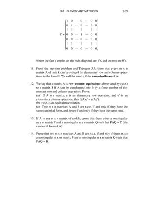
10. Show that an m x n reduced row-echelon matrix R of rank k can be
reduced by elementary column operations to an m x n matrix C of the
form](https://image.slidesharecdn.com/07chap3-150213074831-conversion-gate01/85/07-chap3-54-320.jpg)