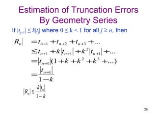
Let's analyze the remainder term R6 using the geometry series method:
|tj+1| = (j+1)π-2 ≤ π-2 = k|tj| for all j ≥ 6 (where 0 < k = π-2 < 1)
Then, |R6| ≤ t7(1 + k + k2 + k3 + ...)
= t7/(1-k)
= 7π-2/(1-π-2)
So the estimated upper bound of the truncation error |R6| is 7π-2/(1-π-2)

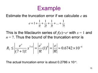
![Analyzing the remainder term of the
Taylor series expansion of f(x)=ex at 0
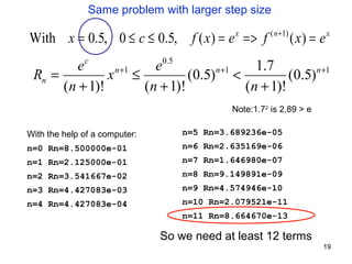
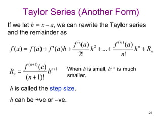
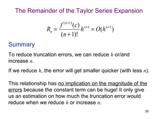
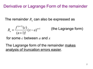
The remainder Rn in the Lagrange form is
( n +1)
f (c )
Rn = ( x − a ) n +1
(n + 1)! for some c between a and x
For f(x) = ex and a = 0, we have f(n+1)(x) = ex. Thus
ec
Rn = x n +1 for some c in [0 , x]
(n + 1)!
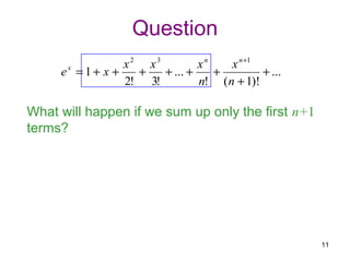
x
e We can estimate the largest possible
≤ x n +1 truncation error through analyzing Rn.
(n + 1)!
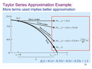
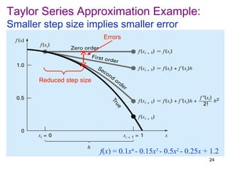
14](https://image.slidesharecdn.com/03truncationerrors-130104021741-phpapp02/85/03-truncation-errors-14-320.jpg)