Downloaded 95 times
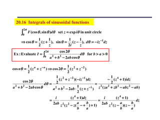
![f ( z ) = u( x , y ) + iv ( x , y ) for z = x + iy
f ( z + ∆z ) − f ( z )
f ' ( z ) = lim [ ] exists
∆z →0 ∆z
Its value does not depend on the direction.
Ex : Show that the function f ( z ) = x 2 − y 2 + i 2 xy is
differentiable for all values of z .
for ∆z = ∆x + i∆y
f ( z + ∆z ) − f ( z )
f ' ( z ) = lim
∆z →0 ∆z
( x + ∆x ) 2 − ( y + ∆y ) 2 + 2i ( x + ∆x )( y + ∆y ) − x 2 + y 2 − 2ixy
=
∆x + i∆y
( ∆x ) 2 − ( ∆y )2 + 2i∆x∆y
= 2x + i2 y +
∆x + i∆y
(1) choose ∆y = 0, ∆x → 0 ⇒ f ' ( z ) = 2 x + i 2 y
(2) choose ∆x = 0, ∆y → 0 ⇒ f ' ( z ) = 2 x + i 2 y](https://image.slidesharecdn.com/complexvarible-121010133525-phpapp01/85/Complex-varible-1-320.jpg)
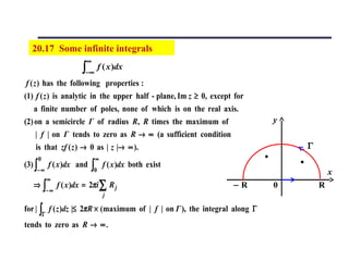
![f ( z ) = u( x , y ) + iv ( x , y ) for z = x + iy
f ( z + ∆z ) − f ( z )
f ' ( z ) = lim [ ] exists
∆z →0 ∆z
Its value does not depend on the direction.
Ex : Show that the function f ( z ) = x 2 − y 2 + i 2 xy is
differentiable for all values of z .
for ∆z = ∆x + i∆y
f ( z + ∆z ) − f ( z )
f ' ( z ) = lim
∆z →0 ∆z
( x + ∆x ) 2 − ( y + ∆y ) 2 + 2i ( x + ∆x )( y + ∆y ) − x 2 + y 2 − 2ixy
=
∆x + i∆y
( ∆x ) 2 − ( ∆y )2 + 2i∆x∆y
= 2x + i2 y +
∆x + i∆y
(1) choose ∆y = 0, ∆x → 0 ⇒ f ' ( z ) = 2 x + i 2 y
(2) choose ∆x = 0, ∆y → 0 ⇒ f ' ( z ) = 2 x + i 2 y](https://image.slidesharecdn.com/complexvarible-121010133525-phpapp01/75/Complex-varible-1-2048.jpg)
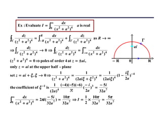
![* * Another method :
f ( z ) = ( x + iy ) 2 = z 2
' ( z + ∆z )2 − z 2 ( ∆z )2 + 2 z∆z
f ( z ) = lim [ ] = lim [ ]
∆z →0 ∆z ∆z → 0 ∆z
= lim ∆z + 2 z = 2 z
∆z → 0
Ex : Show that the function f ( z ) = 2 y + ix is not
differentiable anywhere in the complex plane.
f ( z + ∆z ) − f ( z ) 2 y + 2∆y + ix + i∆x − 2 y − ix 2∆y + i∆x
= =
∆z ∆x + i∆y ∆x + i∆y
if ∆z → 0 along a line thriugh z of slope m ⇒ ∆y = m ∆x
f ( z + ∆z ) − f ( z ) 2 ∆ y + i∆ x 2m + i
f ' ( z ) = lim = lim [ ]=
∆z →0 ∆z ∆x ,∆y →0 ∆x + i∆y 1 + im
The limit depends on m (the direction), so f ( z )
is nowhere differentiable.](https://image.slidesharecdn.com/complexvarible-121010133525-phpapp01/85/Complex-varible-2-320.jpg)
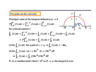
![Ex : Show that the function f ( z ) = 1 /(1 − z ) is analytic everywhere
except at z = 1.
f ( z + ∆z ) − f ( z ) 1 1 1
f ' ( z ) = lim [ ] = lim [ ( − )]
∆z →0 ∆z ∆z →0 ∆z 1 − z − ∆z 1 − z
1 1
= lim [ ]=
∆z →0 (1 − z − ∆z )(1 − z ) (1 − z ) 2
Provided z ≠ 1, f ( z ) is analytic everywhere such that
f ' ( z ) is independent of the direction.](https://image.slidesharecdn.com/complexvarible-121010133525-phpapp01/85/Complex-varible-3-320.jpg)
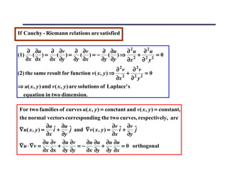
![20.2 Cauchy-Riemann relation
A function f(z)=u(x,y)+iv(x,y) is differentiable and analytic,
there must be particular connection between u(x,y) and v(x,y)
f ( z + ∆z ) − f ( z )
L = lim [ ]
∆z →0 ∆z
f ( z ) = u( x , y ) + iv ( x , y ) ∆z = ∆x + i∆y
f ( z + ∆z ) = u( x + ∆x , y + ∆y ) + iv ( x + ∆x , y + ∆y )
u( x + ∆x , y + ∆y ) + iv ( x + ∆x , y + ∆y ) − u( x , y ) − iv ( x , y )
⇒ L = lim [ ]
∆x ,∆y →0 ∆x + i∆y
(1) if suppose ∆z is real ⇒ ∆y = 0
u( x + ∆x , y ) − u( x , y ) v ( x + ∆x , y ) − v ( x , y ) ∂u ∂v
⇒ L = lim [ +i ]= +i
∆x →0 ∆x ∆x ∂x ∂x
(2) if suppose ∆z is imaginary ⇒ ∆x = 0
u( x , y + ∆y ) − u( x , y ) v ( x , y + ∆y ) − v ( x , y ) ∂u ∂v
⇒ L = lim [ +i ] = −i +
∆y →0 i ∆y i ∆y ∂y ∂y
∂u ∂v ∂v ∂u
= and =- Cauchy - Riemann relations
∂x ∂y ∂x ∂y](https://image.slidesharecdn.com/complexvarible-121010133525-phpapp01/85/Complex-varible-4-320.jpg)
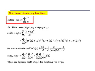
![Ex : In which domain of the complex plane is
f ( z ) =| x | − i | y | an analytic function?
u( x , y ) =| x |, v ( x , y ) = − | y |
∂u ∂v ∂ ∂
(1) = ⇒ | x |= [− | y |] ⇒ (a) x > 0, y < 0 the fouth quatrant
∂x ∂y ∂x ∂y
(b) x < 0, y > 0 the second quatrant
∂v ∂u ∂ ∂
(2) =− ⇒ [− | y |] = − | x |
∂x ∂y ∂x ∂y
z = x + iy and complex conjugate of z is z * = x − iy
⇒ x = ( z + z * ) / 2 and y = ( z − z * ) / 2i
∂f ∂f ∂x ∂f ∂y 1 ∂u ∂v i ∂v ∂u
⇒ = + = ( − )+ ( + )
∂z * ∂x ∂z * ∂y ∂z * 2 ∂x ∂y 2 ∂x ∂y
If f ( z ) is analytic , then the Cauchy - Riemann relations
are satisfied. ⇒ ∂f / ∂z * = 0 implies an analytic fonction of z contains
the combination of x + iy , not x − iy](https://image.slidesharecdn.com/complexvarible-121010133525-phpapp01/85/Complex-varible-5-320.jpg)

![Set exp w = z
Write z = r exp iθ for r is real and − π < θ ≤ π
⇒ z = r exp[i (θ + 2nπ )] ⇒ w = Lnz = ln r + i (θ + 2nπ )
Lnz is a multivalued function of z .
Take its principal value by choosing n = 0
⇒ ln z = ln r + iθ -π < θ ≤ π
If t ≠ 0 and z are both complex numbers, we define
t z = exp( zLnt )
Ex : Show that there are exactly n distinct nth roots of t .
1
1
tn = exp( Lnt ) and t = r exp[i (θ + 2kπ )]
n
1 1
1 (θ + 2kπ ) (θ + 2kπ )
⇒ tn = exp[ ln r + i ] = r n exp[i ]
n n n](https://image.slidesharecdn.com/complexvarible-121010133525-phpapp01/85/Complex-varible-10-320.jpg)
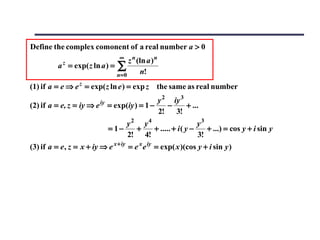
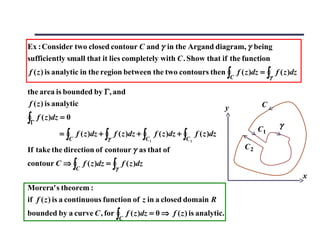
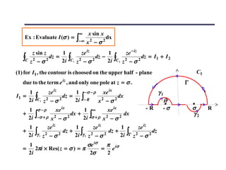
![20.5 Multivalued functions and branch cuts
A logarithmic function, a complex power and a complex root are all
multivalued. Is the properties of analytic function still applied?
Ex : f ( z ) = z 1 / 2 and z = r exp(iθ ) (A) C
y
(A) z traverse any closed contour C that
dose not enclose the origin, θ return r
to its original value after one complete θ
x
circuit.
(B) y
(B) θ → θ + 2π enclose the origin
C' r
1/ 2 1/ 2
r exp(iθ / 2) → r exp[i (θ + 2π ) / 2]
θ
= − r 1 / 2 exp(iθ / 2) x
⇒ f (z) → − f (z)
z = 0 is a branch point of the function f ( z ) = z 1 / 2](https://image.slidesharecdn.com/complexvarible-121010133525-phpapp01/85/Complex-varible-11-320.jpg)

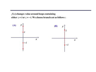
![Ex : Find the branch points of f ( z ) = z 2 + 1 , and hence sketch
suitable arrangements of branch cuts.
f ( z ) = z 2 + 1 = ( z + i )( z − i ) expected branch points : z = ± i
set z − i = r1 exp(iθ1 ) and z + i = r2 exp(iθ 2 )
⇒ f ( z ) = r1r2 exp(iθ1 / 2) exp(iθ 2 / 2)
= r1r2 exp[i (θ1 + θ 2 )]
If contour C encloses
(1) neither branch point, then θ1 → θ1 , θ 2 → θ 2 ⇒ f ( z ) → f ( z )
(2) z = i but not z = − i , then θ1 → θ1 + 2π , θ 2 → θ 2 ⇒ f ( z ) → − f ( z )
(3) z = − i but not z = i , then θ1 → θ1 , θ 2 → θ 2 + 2π ⇒ f ( z ) → − f ( z )
(4) both branch points, then θ1 → θ1 + 2π ,θ 2 → θ 2 + 2π ⇒ f ( z ) → f ( z )](https://image.slidesharecdn.com/complexvarible-121010133525-phpapp01/85/Complex-varible-13-320.jpg)
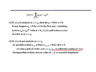
![20.6 Singularities and zeros of complex function
g( z )
Isolated singularity (pole) : f ( z ) =
( z − z0 ) n
n is a positive integer, g( z ) is analytic at all points in
some neighborhood containing z = z0 and g( z0 ) ≠ 0,
the f ( z ) has a pole of order n at z = z0 .
* * An alternate definition for that f ( z ) has a pole of
order n at z = z0 is
lim [( z − z0 ) n f ( z )] = a
z → z0
f ( z ) is analytic and a is a finite, non - zero complex number
(1) if a = 0, then z = z0 is a pole of order less than n.
(2) if a is infinite, then z = z0 is a pole of order greater than n.
(3) if z = z0 is a pole of f ( z ) ⇒| f ( z ) |→ ∞ as z → z0
(4) from any direction, if no finite n satisfies the limit ⇒ essential singularity](https://image.slidesharecdn.com/complexvarible-121010133525-phpapp01/85/Complex-varible-15-320.jpg)
![Ex : Find the singularities of the function
1 1
(1) f ( z ) = −
1− z 1+ z
2z
⇒ f (z) = poles of order 1 at z = 1 and z = −1
(1 − z )(1 + z )
(2) f ( z ) = tanh z
sinh z exp z − exp(− z )
= =
cosh z exp z + exp(− z )
f ( z ) has a singularity when exp z = − exp(− z )
⇒ exp z = exp[i ( 2n + 1)π ] = exp(− z ) n is any integer
1
⇒ 2 z = i ( 2n + 1)π ⇒ z = ( n + )πi
2
Using l' Hospital' s rule
[ z − ( n + 1 / 2)πi ] sinh z [ z − ( n + 1 / 2)πi ] cosh z + sinh z
lim { }= lim { }=1
z →( n+1 / 2 )πi cosh z z →( n+1 / 2 )πi sinh z
each singularity is a simple pole (n = 1)](https://image.slidesharecdn.com/complexvarible-121010133525-phpapp01/85/Complex-varible-16-320.jpg)
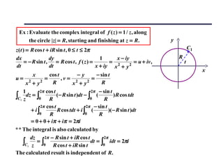
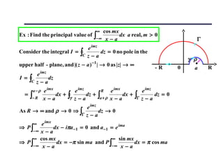
![Ex : Evaluate the complex integral of f ( z ) = 1 / z along
(i) the contour C 2 consisting of the semicircle | z |= R in
the half - plane y ≥ 0
(ii) the contour C 3 made up of two straight lines C 3a and C 3b
(i) This is just as in the previous example, but for
y
0 ≤ t ≤ π ⇒ ∫ dz / z = πi iR
C2
C 3b
(ii) C 3a : z = (1 − t ) R + itR for 0 ≤ t ≤ 1 C 3a
C 3b : − sR + i (1 − s ) R for 0 ≤ s ≤ 1 s=1 t=0
dz 1 − R + iR 1 − R − iR −R R x
∫C3 z 0 R + t (− R + iR) 0 iR + s(− R − iR)
=∫ dt + ∫ dt
1 −1+ i 1 2t − 1 1 1
1st term ⇒ ∫ dt = ∫ dt + i ∫ dt
0 1 − t + it 0 1 − 2 t + 2t 2 0 1 − 2t + 2t 2
1 i t −1/ 2 1
= [ln(1 − 2t + 2t 2 )] |1 + [2 tan −1 (
0 )] |0
2 2 1/ 2
i π π πi a x
= 0 + [ − ( − )] = ∫ a2 + x2 dx = tan −1 ( ) + c
2 2 2 2 a](https://image.slidesharecdn.com/complexvarible-121010133525-phpapp01/85/Complex-varible-22-320.jpg)
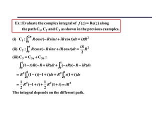
![1 1+ i 1 (1 + i )[ s − i ( s − 1)]
2nd term ⇒ ∫ ds = ∫ ds
0 s + i ( s − 1) 0 2
s + ( s − 1) 2
1 2s − 1 1 1
=∫ ds + i ∫ ds
0 2s 2 − 2s + 1 0 2s 2 − 2s + 1
1 s −1/ 2 1
= [ln( 2 s 2 − 2 s + 1)] |1 + i tan −1 (
0 ) |0
2 1/ 2
π π πi
= 0 + i[ − ( − )] =
4 4 2
dz
⇒ ∫C3 z = πi
The integral is independent of the different path.](https://image.slidesharecdn.com/complexvarible-121010133525-phpapp01/85/Complex-varible-23-320.jpg)
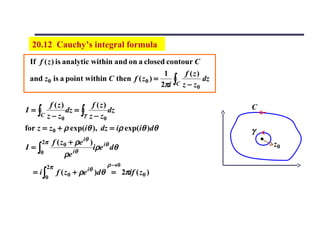
![20.11 Cauchy theorem
If f ( z ) is an analytic function, and f ' ( z ) is continuous
at each point within and on a closed contour C
⇒ ∫ f ( z )dz = 0
C
∂p( x , y ) ∂q( x , y )
If and are continuous within and
∂x ∂y
on a closed contour C, then by two - demensional
∂p ∂q
divergence theorem ⇒ ∫∫ ( + )dxdy = ∫ ( pdy − qdx )
R ∂x ∂y C
f ( z ) = u + iv and dz = dx + idy
I = ∫ f ( z )dz = ∫ ( udx − vdy ) + i ∫ (vdx + udy )
C C C
∂ ( − u) ∂ ( − v ) ∂ ( − v ) ∂u
= ∫∫ [ + ]dxdy + i ∫∫ [ + ]dxdy = 0
R ∂y ∂x R ∂y ∂x
f ( z ) is analytic and the Cauchy - Riemann relations apply.](https://image.slidesharecdn.com/complexvarible-121010133525-phpapp01/85/Complex-varible-25-320.jpg)
![The integral form of the derivative of a complex function :
1 f (z)
f ' ( z0 ) =
2πi ∫C ( z − z )2 dz
0
f ( z 0 + h) − f ( z 0 )
f ' ( z0 ) = lim
h→ 0 h
1 f (z) 1 1
= lim [
h→0 2πi
∫C h z − z0 − h z − z0 )dz ]
( −
1 f (z)
= lim [
h→ 0 2πi ∫C ( z − z0 − h)( z − z0 )dz ]
1 f (z)
=
2πi ∫C ( z − z )2 dz
0
n! f (z)
2πi ∫C ( z − z0 )n+1
For nth derivative f ( n ) ( z0 ) = dz](https://image.slidesharecdn.com/complexvarible-121010133525-phpapp01/85/Complex-varible-29-320.jpg)
![1
Ex : Find the Laurent series of f ( z ) = 3
about the singularities
z ( z − 2)
z = 0 and z = 2. Hence verify that z = 0 is a pole of order 1 and z = 2 is a
pole of order 3, and find the residue of f ( z ) at each pole.
(1) point z = 0
−1 −1 − z ( −3)( −4) − z 2 ( −3)( −4)( −5) − z 3
f (z) = 3
= [1 + ( −3)( ) + ( ) + ( ) + ...]
8 z (1 − z / 2) 8z 2 2! 2 3! 2
1 3 3 5z 2
=− − − z− − ... z = 0 is a pole of order 1
8 z 16 16 32
(2) point z = 2 ⇒ set z − 2 = ξ ⇒ z( z − 2) 3 = ( 2 + ξ )ξ 3 = 2ξ 3 (1 + ξ / 2)
1 1 ξ ξ ξ ξ
f (z) = 3 = 3 [1 − ( ) + ( )2 − ( )3 + ( )4 − ...]
2ξ (1 + ξ / 2) 2ξ 2 2 2 2
1 1 1 1 ξ 1 1 1 1 z−2
= − + − + − .. = − + − + −
2ξ 3
4ξ 2 8ξ 16 32 2( z − 2) 3
4( z − 2) 2 8( z − 2) 16 32
z = 2 is a pole of order 3, the residue of f ( z ) at z = 2 is 1 / 8.](https://image.slidesharecdn.com/complexvarible-121010133525-phpapp01/85/Complex-varible-34-320.jpg)
![How to obtain the residue ?
a− m a−1
f (z) = + ...... + + a0 + a1 ( z − z0 ) + a 2 ( z − z0 )2 + ...
( z − z0 ) m ( z − z0 )
⇒ ( z − z0 )m f ( z ) = a − m + a − m +1 ( z − z0 ) + ....... + a −1 ( z − z0 )m −1 + ...
d m −1 ∞
⇒ m −1
[( z − z0 ) f ( z )] = ( m − 1)! a −1 + ∑ bn ( z − z0 )n
m
dz n =1
Take the limit z → z0
1 d m −1
R( z0 ) = a −1 = lim { [( z − z0 ) m f ( z )]} residue at z = z0
z → z0 ( m − 1)! dz m −1
(1) For a simple pole m = 1 ⇒ R( z0 ) = lim [( z − z0 ) f ( z )]
z → z0
g( z )
(2) If f ( z ) has a simple at z = z0 and f ( z ) = , g ( z ) is analytic and
h( z )
non - zero at z0 and h( z0 ) = 0
( z − z0 ) g ( z ) ( z − z0 ) 1 g( z )
⇒ R( z0 ) = lim = g ( z0 ) lim = g ( z0 ) lim ' = ' 0
z → z0 h( z ) z → z0 h( z ) z → z0 h ( z ) h ( z0 )](https://image.slidesharecdn.com/complexvarible-121010133525-phpapp01/85/Complex-varible-35-320.jpg)
![Ex : Suppose that f ( z ) has a pole of order m at the point z = z0 . By
considering the Laurent series of f ( z ) about z0 , deriving a general
expression for the residue R( z0 ) of f ( z ) at z = z0 . Hence evaluate
exp iz
the residue of the function f ( z ) = 2 2
at the point z = i .
( z + 1)
exp iz exp iz
f (z) = 2 2
= 2 2
poles of order 2 at z = i and z = − i
( z + 1) (z + i) (z − i)
for pole at z = i :
d d exp iz i 2
[( z − i ) 2 f ( z )] = [ 2
]= 2
exp iz − 3
exp iz
dz dz ( z + i ) (z + i) (z + i)
1 i 2 −i
R( i ) = [ e −1 − e −1 ] =
1! ( 2i ) 2 ( 2i ) 3 2e](https://image.slidesharecdn.com/complexvarible-121010133525-phpapp01/85/Complex-varible-36-320.jpg)
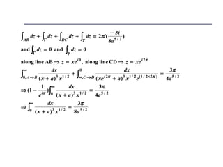
![i z4 + 1
2ab ∫C
I= dz double poles at z = 0 and z = a / b within the unit circle
a b
z 2 ( z − )( z − )
b a
1 d m −1
Residue : R( z0 ) = lim { [( z − z0 ) m f ( z )]
z → z0 ( m − 1)! dz m −1
(1) pole at z = 0, m = 2
1 d 2 z4 + 1
R(0) = lim { [z 2 ]}
z →0 1! dz z ( z − a / b )( z − b / a )
4z 3 ( z 4 + 1)( −1)[2 z − (a / b + b / a )]
= lim { + }= a/b+b/a
z →0 ( z − a / b )( z − b / a ) 2
( z − a / b) ( z − b / a ) 2
(2) pole at z = a / b, m = 1
z4 + 1 (a / b)4 + 1 − (a 4 + b 4 )
R(a / b) = lim [( z − a / b ) 2
]= 2
=
z →a / b z ( z − a / b )( z − b / a ) (a / b) (a / b − b / a ) ab(b 2 − a 2 )
i a 2 + b2 a 4 + b4 2πa 2
I = 2πi × [ − ]= 2 2
2ab ab ab(b − a ) b (b − a 2 )
2 2](https://image.slidesharecdn.com/complexvarible-121010133525-phpapp01/85/Complex-varible-41-320.jpg)
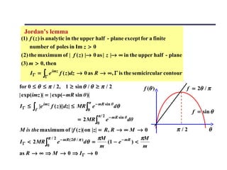
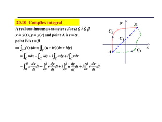
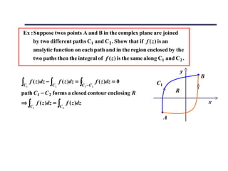
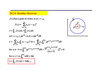
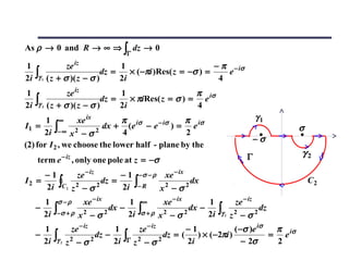
![20.18 Integral of multivalued functions
1/ 2
y
Multivalued functions such as z , Lnz
Single branch point is at the otigin. We let R → ∞ R Γ
and ρ → 0. The integrand is multivalued, its values
γ
along two lines AB and CD joining z = ρ to z = R A B
are not equal and opposite. ρ x
C D
∞ dx
Ex : I = ∫0 ( x + a )3 x1 / 2
for a > 0
(1) the integrand f ( z ) = ( z + a ) −3 z −1 / 2 , |zf ( z )| → 0 as ρ → 0 and R → ∞
the two circles make no contribution to the contour integral
(2) pole at z = − a , and ( − a )1 / 2 = a 1 / 2 e iπ / 2 = ia 1 / 2
1 d 3 −1 1
R( − a ) = lim [( z + a )3 ]
z → − a ( 3 − 1)! dz 3 − 1 3 1/ 2
(z + a) z
1 d 2 −1 / 2 − 3i
= lim z =
z → − a 2! dz 2 8a 5 / 2](https://image.slidesharecdn.com/complexvarible-121010133525-phpapp01/85/Complex-varible-47-320.jpg)

The document discusses complex differentiability and analytic functions. It shows that for a function f(z) to be complex differentiable, the Cauchy-Riemann equations relating the partial derivatives of the real and imaginary parts must be satisfied. It also discusses representing functions as power series and their radii of convergence. Multivalued functions like logarithms and roots are discussed, noting the need for branch cuts to define single-valued branches.