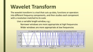
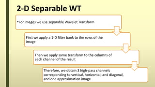
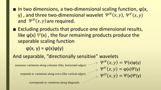
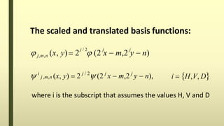
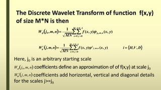
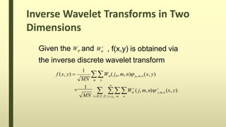
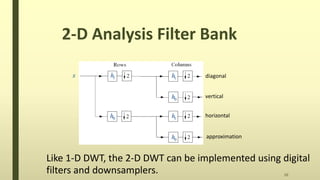
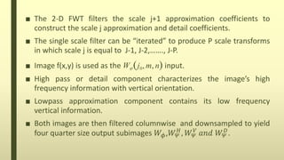
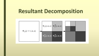
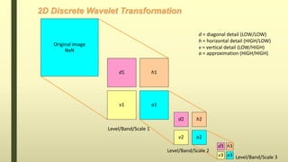
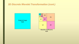
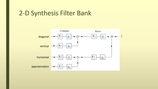
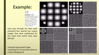
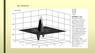
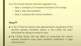
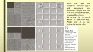
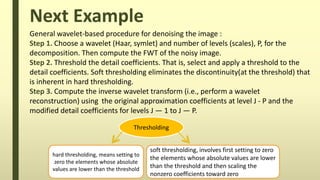
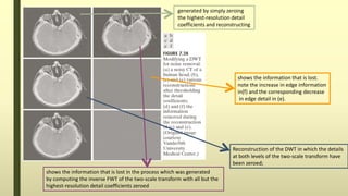
The document discusses the wavelet transform in two dimensions. It begins by explaining that the wavelet transform decomposes data into different frequency components using variable length windows tailored to each scale. For image processing, two-dimensional wavelets are required. The two-dimensional wavelet transform can be implemented using separable filters that are applied first along rows then columns. This results in approximation, horizontal, vertical and diagonal detail coefficients. The document provides examples of applying the two-dimensional discrete wavelet transform to images and discusses applications such as denoising.

1. WAVELET TRANSFORM
IN TWO DIMENSIONS
Presented By:
Ayushi Gagneja

2. Wavelet Transform
The wavelet transform is a tool that cuts up data, functions or operators
into different frequency components, and then studies each component
with a resolution matched to its scale
Uses a variable length window, e.g.:
Narrower windows are more appropriate at high frequencies
Wider windows are more appropriate at low frequencies

3. Wavelet Functions
■ Different purposes, different wavelets

4. Two-Dimensional Wavelets
• For image processing applications we need
wavelets that are two-dimensional.
• This problem reduces down to designing 2D filters.
• We will focus on a particular class of 2D filters:
separable filters (can be directly designed from
their 1D counterparts)

5. 2-D Separable WT
•For images we use separable Wavelet Transform
First we apply a 1-D filter bank to the rows of the
image
Then we apply same transform to the columns of
each channel of the result
Therefore, we obtain 3 high-pass channels
corresponding to vertical, horizontal, and diagonal,
and one approximation image

6. ■ In two dimensions, a two-dimensional scaling function, ϕ(x,
y) , and three two-dimensional wavelet ,
and are required.
■ Excluding products that produce one dimensional results,
like ϕ(x) 𝛹(x) , the four remaining products produce the
separable scaling function
ϕ(x, y) = ϕ(x)ϕ(y)
And separable, “directionally sensitive” wavelets
𝛹 𝐻
𝑥, 𝑦 𝛹 𝑉
𝑥, 𝑦
𝛹 𝐷
𝑥, 𝑦
𝛹 𝐻
𝑥, 𝑦 = 𝛹(x)ϕ(y)
𝛹 𝑉 𝑥, 𝑦 = ϕ(x)𝛹(y)
𝛹 𝐷
𝑥, 𝑦 = 𝛹(x)𝛹(y)
corresponds to variations along diagonals
measures variations along columns (like, horizontal edges)
responds to variations along rows (like vertical edges)

7. The scaled and translated basis functions:
j / 2 j j
 j,m,n (x, y) 2  (2 x  m,2 y  n)
i  H,V, D i
j,m,n (x, y)  2 j / 2
 (2 j
x  m,2 j
y  n),
where i is the subscript that assumes the values H, V and D

8. The Discrete Wavelet Transform of function f(x,y)
of size M*N is then
1 M 1N 1
x0 y 0MN
Wj0 ,m,n  f (x, y) j0 ,m,n (x, y)
1 M 1N 1
x0 y 0
i
i  H,V, D
MN
W j,m,n  f (x, y) i
j ,m,n (x, y)
Here, j0 is an arbitrary starting scale
Wj0,m,n coefficients define an approximation of of f(x,y) at scale j0
coefficients add horizontal, vertical and diagonal details
for the scales j>=j0
i
W j, m,n

9. , f(x,y) is obtained via
the inverse discrete wavelet transform
i
Given the W and W

i
m n
MN iH ,V ,D j j m n
i
j,m,n
0
(x, y)
MN

1
1
W ( j, m,n)  
f (x, y)  W ( j0, m, n)j0 ,m,n (x, y)
Inverse Wavelet Transforms in Two
Dimensions

10. 2-D Analysis Filter Bank
10
1h
0h
1h
1h
0h
0h
x diagonal
vertical
horizontal
approximation
Like 1-D DWT, the 2-D DWT can be implemented using digital
filters and downsamplers.

11. ■ The 2-D FWT filters the scale j+1 approximation coefficients to
construct the scale j approximation and detail coefficients.
■ The single scale filter can be “iterated” to produce P scale transforms
in which scale j is equal to J-1, J-2,……., J-P.
■ Image f(x,y) is used as the W j0, m, n input.
■ High pass or detail component characterizes the image’s high
frequency information with vertical orientation.
■ Lowpass approximation component contains its low frequency
vertical information.
■ Both images are then filtered columnwise and downsampled to yield
four quarter size output subimages 𝑊𝜙,𝑊 𝛹
𝐻
, 𝑊 𝛹
𝑉
𝑎𝑛𝑑 𝑊 𝛹
𝐷
.

12. Resultant Decomposition

13. 2D Discrete Wavelet Transformation
d2 h2
v2 a2
a1
h1d1
v1
Original image
NxN
a3
d3 h3
v3
Level/Band/Scale 1
Level/Band/Scale 2
Level/Band/Scale 3
d = diagonal detail (LOW/LOW)
h = horizontal detail (HIGH/LOW)
v = vertical detail (LOW/HIGH)
a = approximation (HIGH/HIGH)

14. 2D Discrete Wavelet Transformation (cont.)
d2
h2
v2
h1
d1v1
a3
d3
h3
v3
Original image
NxN
Wavelet coefficients
NxN

15. 2-D Synthesis Filter Bank
ˆxdiagonal
vertical
horizontal
approximation
1g
1g
1g
0g
0g
0g

16. ■ Synthesis Filter bank reverses the process.
■ At each iteration, four scale j approximation and detail
subimages are upsampled and convolved with the 2-D
filters, one operating on subimages columns and other
on its rows.
■ Addition of the results yields the scale j+1
approximation, and process is repeated until the
original image is reconstructed.

17. computer-generated image
consisting of 2-D sine-like pulses on
a black background
Each pass through the filter bank
produced four quarter-size output
images that were substituted for
the input from which they were
derived.
Example:

18. Next example
• The decomposition filters used in the preceding example are
part of a well known family of wavelets called symlets, short
for "symmetrical wavelets.“
• Figure 7.26(a) and (d), shows the corresponding
decomposition and reconstruction filters.
• The coefficients of lowpass reconstruction filter go(n) = hφ(n)
for 0 < n < 7 .
• Figure 7.26(g), a low-resolution graphic depiction of wavelet
𝛹 𝑣 𝑥, 𝑦 , is provided as an illustration of how a one-
dimensional scaling and wavelet function can combine to
form a separable, two-dimensional wavelet .

20. Fig. 7.26 (Con’t)

21. As in the Fourier domain, the basic approach is to
– Step 1. Compute a 2-D wavelet transform of an image.
– Step 2. Alter the transform.
– Step 3. Compute the inverse transform.
How??
■ In Fig 7.27(a) the lowest scale approximation component of the
discrete wavelet transform shown in Fig 7.25(c) has been
eliminated by setting its values to zero.
■ Fig 7.27(b) shows, the net effect of computing the inverse
wavelet transform using these modified coefficients is edge
enhancement.

22. Note how well the
transitions between signal
and background are
delineated, despite the fact
that they are relatively soft,
sinusoidal transitions.
By zeroing the horizontal
details as well—see Figs.
7.27(c) and (d)—we can
isolate the vertical edges .

23. Next Example
Thresholding
hard thresholding, means setting to
zero the elements whose absolute
values are lower than the threshold
soft thresholding, involves first setting to zero
the elements whose absolute values are lower
than the threshold and then scaling the
nonzero coefficients toward zero
General wavelet-based procedure for denoising the image :
Step 1. Choose a wavelet (Haar, symlet) and number of levels (scales), P, for the
decomposition. Then compute the FWT of the noisy image.
Step 2. Threshold the detail coefficients. That is, select and apply a threshold to the
detail coefficients. Soft thresholding eliminates the discontinuity(at the threshold) that
is inherent in hard thresholding.
Step 3. Compute the inverse wavelet transform (i.e., perform a wavelet
reconstruction) using the original approximation coefficients at level J - P and the
modified detail coefficients for levels J — 1 to J — P.

24. shows the information that is lost.
note the increase in edge information
in(f) and the corresponding decrease
in edge detail in (e).
generated by simply zeroing
the highest-resolution detail
coefficients and reconstructing
shows the information that is lost in the process which was generated
by computing the inverse FWT of the two-scale transform with all but the
highest-resolution detail coefficients zeroed
Reconstruction of the DWT in which the details
at both levels of the two-scale transform have
been zeroed;

25. Wavelets Applications
Feature Extraction
Hardware Implementation
Document Analysis
Classification
Image matching and retrieval
Recognition
Image compression
•Noise filtering

26. THANK YOU