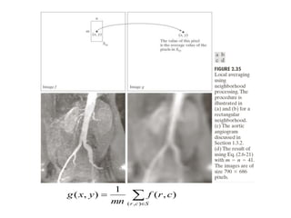
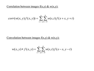
This document discusses basics of intensity transformations and spatial filtering of digital images. It covers the following key points: - Intensity transformations map input pixel intensities to output intensities using an operator T. Common transformations include log, power-law, and piecewise-linear functions. - Spatial filters operate on neighborhoods of pixels. Linear filters perform averaging or correlation while non-linear filters use ordering like median. - Basic filters include smoothing to reduce noise, sharpening to enhance edges using Laplacian or unsharp masking, and gradient for edge detection. - Fuzzy set theory can be applied to intensity transformations by defining membership functions for concepts like dark/bright. It can also be used for spatial filtering by defining

1.  Basics of Intensity Transformations and Spatial Filtering
g(x,y) = T [f(x,y)]
where f(x,y) is the input image, g(x,y) is the output image, and T is
an operator on f defined over a neighborhood of point (x,y)

2. 

Scr
crf
mn
yxg
),(
),(
1
),(

3. a) median filtering b) Average filtering

4.  Procedure discussed is known as Spatial filtering.
 Filter is referred as spatial filter, and also referred as spatial mask,
kernel, template or window.
 The type of operation performed in the neighborhood determines
the nature of filtering process.
 Intensity (gray level or mapping) transformation function
s=T(r)
s and r are variables denoting intensity of g and f at any point
(x,y)

5. BASIC INTENSITY TRANSFORMATION FUNCTIONS:
 Image negatives
The negative of an image with intensity levels in the range[0,L-1]
is obtained by using the negative transformation, given by the expression:
s = L-1-r
reversing the intensity levels of an image in this manner produce
the equivalent of a photographic negative.
 Log Transformations
The general form of log transformation is
s = c log(1+r)
where c is constant & assumed that r ≥ 0.
This transformation maps a narrow range of low intensity values in the point
into a wider range of output values.
 nth root and nth power transformations.

7. Power-Law(Gamma) Transformations:
This transformations have the basic form as
Where c and ϒ are positive constants
A variety of devices used for image capture, printing and display
respond according to power law.
Eg: CRT devices have an intensity to voltage response , i.e., a power
function

crs 

11. Piecewise-Linear Transformation Functions:
1) Contrast Stretching:
Because of poor illumination, lack of dynamic range in the imaging
sensor, or even the wrong settings of lens aperture during acquisition, it results
to low contrast images.
Contrast stretching is a process that expands the range of intensity
levels in an image so that it spans the full intensity range of the recording
medium or display device.

12. Intermediate values of produce various degrees of spread in
intensity levels of the output image, thus effecting its contrast. In general
is assumed & this condition preserves the order of intensity levels
thus preventing the creation of intensity artifacts in the processed image
),(),( 2211 srandsr
2121 , ssrr 

13. 2) Intensity level slicing:
 Highlighting a specific range of intensities in an image often is of interest
 Applications include enhancing features such as masses of water in satellite
imaging and enhancing flaws in X-ray images.

15. 3) Bit plane slicing:
Pixels are digital numbers composed of bits. The intensity of each
pixel in a 256 level gray scale image is composed of 8 bits.
Instead of highlighting intensity level ranges, we could highlight the
contribution made to total image appearance by specific bits.
An 8 bit image may be considered as being composed of 8 1-bit planes, with
plane 1 containing the lowest –order bit of all pixels in the image and plane 8
all the highest-order bits.

16.  Decomposing an image into bit planes is useful for analyzing the relative
importance of each bit in the image.
 This type of decomposition is useful for image compression, in which fewer
than all planes are used in reconstructing an image.

18. Histogram:
• The histogram of a digital image with intensity levels in the range
[0,L-1] is a discrete function h(rk)= nk , where rk is the kth intensity
value and nk is the no. of pixels in the image of intensity rk .
• Normalized histogram is given by
p(rk)= nk /MN, for k = 0,1,2,…(L-1)
• p(rk) is an estimate of the probability of occurrence of intensity
level rk in an image.
• The sum of all components of a normalized histogram is equal to 1

20. Histogram Equalization:
Consider for a moment continuous intensity values and let the
variable r denote the intensities of an image to be processed. We assume
that r is in the range [0, L-1], with r=0 (black) and r=L-1 (white). For r
satisfying these conditions. We focus on attention on transformations of
the form
s = T(r) , 0 ≤ r ≤L-1
that produce an output intensity level s for every pixel in the input image
having intensity r. We assume that:
a) T(r) is a monotonically increasing function in the interval 0 ≤ r ≤ L-1
b) 0 ≤ T(r) ≤ L-1 for 0 ≤ r ≤ L-1

21. In some formulations to be discussed later, we use the inverse
r=T -1(s) ; 0 ≤ s ≤ L-1
in which case we change condition (a) to (a1)
i.e, T(r) is a strictly monotonically increasing function in the interval
0 ≤ r ≤ L-1

26. Example: suppose that a 3-bit image(L=8) of size 64x64(MN=4096) has the
intensity distribution as shown in below table

27. These are the values of equalised histogram. Original image 8 intensity levels are
mapped to 5 distinct intensity levels.

29. SPATIAL FILTERING

31.  Spatial filter consists of
i) neighborhood
ii) a predefined operation that is performed on the image pixels
encompassed by the neighborhood.
Filtering creates a new pixel with coordinates equal to the
coordinates of the center of neighborhood, and whose value is the
result of filtering operation.
 If the operation performed on the image pixels is linear, then the
filter is called a linear spatial filter. Otherwise the filter is nonlinear.
)1,1()1,1(...),()0,0(
...),1()0,1()1,1()1,1(),(


yxfwyxfw
yxfwyxfwyxg

32. For mask of size m x n, we assume that m=2a+1, n=2b+1, where a,b are
positive integers. we concentrate on the filters of odd size.
linear spatial filtering of an image of size MxN with a filter of size m x nis
given by,
Where x and y are varied so that each pixel in w visits every pixel in f.
  

a
as
b
bt
tysxftswyxg ),(),(),(

35. Correlation between images f(x,y) & w(x,y):
Convolution between images f(x,y) & w(x,y):
  

a
as
b
bt
tysxftswyxfyxwcorr ),(),()),(),((
  

a
as
b
bt
tysxftswyxfyxw ),(),(),(),(

36. Smoothing Spatial Filters
1) Smoothing Linear filters:
 the output of smoothing, linear filter is simply the avg. Of the pixels
contained in the neighbourhood of the filter mask.
These filters sometimes called averaging filters.
Reduces sharp transitions in image intensities.
Most obvious application of smoothing is noise reduction.
Smoothing of false contours(because of insufficient no.of intensities)
Undesirable side effect: blur edges

37. A spatial averaging filter in which all coefficients are equal sometimes
is called a box filter.
General implementation for filtering an M x N image with a weighted
averaging filter of size m x n is given by expression,


 
 

 a
as
b
bt
a
as
b
bt
tsw
tysxftsw
yxg
),(
),(),(
),(

38. Order static (nonlinear) filters:
Non linear filters whose response is based on ordering the pixels
contained in image area.
The best known filter in this category is median filter.
They provide excellent noise reduction capabilities.
Considerably less blurring than linear smoothing filters.
Particularly effective in presence of impulse noise.
Other examples: max filter, min filter etc.,

40. Sharpening Spatial Filters
Objective of sharpening is to highlight transitions in
intensities.
Applications ranging from electronic printing and medical
imaging to industrial inspection and autonomous guidance in
military systems.
Sharpening filters are based on first and second order
derivatives

42. • Edges in digital images often are ramp like transitions in intensity, in
which case the 1st derivative of the image would result in thick
edges, because the derivative is non zero along the ramp.
• 2nd derivative would produce a double edge one pixel thick,
separated by zeros. This enhances fine detail much better than 1st
derivative, and ideally suited for sharpening images.
The Laplacian: 2nd order derivative tool for image sharpening
2 2
2
2 2
( , )
( 1, ) ( 1, ) ( , 1) ( , 1) 4 ( , )
f f
f x y
x y
f x y f x y f x y f x y f x y
 
  
 
        

45. Unsharp Masking and Highboost filtering
 Process used in printing and publishing industry.
 Unsharp Masking: Subtracting an unsharp(smoothed) version of
an image from the original image.
Steps for unsharp masking:
1) Blur the original image
2) Subtract the blurred image from the original(result is mask).
3) Add the mask to original.
Let f̅(x,y) denote the blurred image, first we obtain the mask:
gmask (x,y)=f(x,y) - f̅(x,y)
Then add weighted portion of the mask back to the original image
g(x,y) = f(x,y) + k . gmask (x,y)
When k=1, we have unsharp masking.
When k > 1, it is referred to as highboost filtering.

47. The Gradient- using 1st order derivative for image sharpening:
First derivatives in image processing are implemented using the
magnitude of the gradient. For a function f(x,y) the gradient of f at
coordinates (x,y) is defined as the two dimensional column vector.
This vector has the important geometrical property that it points in the
direction of the greatest rate of change of f at location (x,y).
The magnitude of vector ∇f , denoted as M(x,y), where
M(x,y) is the value at (x,y) of the rate of change in the direction of the
gradient vector























y
f
x
f
g
g
fgradf
y
x
)(
22
)(),( yx ggfmagyxM 

50. PRINCIPLES OF FUZZY SET THEORY:
Let Z be the set of elements with generic element of Z denoted by z, i.e. Z={z}. This set is
called universe of discourse. A fuzzy set, A in Z is characterized by a membership
function, μA(z), that associates with each element of Z a real number in the interval [0 1].
The value of μA(z) at z represents the grade of membership of z in A.
With fuzzy sets, we say that all z s for which μA(z) =1 are full members of the set.
all z s for which μA(z) =0 are not members of the set.
all zs for which μA(z) = between 0 &1 have partial membership in the set.
A={z, μA(z) |z ϵ Z }

52. Types of membership functions used in practice. Triangular, Trapezoidal and Sigma
functions are piecewise linear, S & bell shape fns. are smooth. S shape fn. is used
frequently when working with fuzzy sets. The value of z=b is called crossover point.

53. The problem specific knowledge just explained can be formalized in the
form of the following fuzzy IF-THEN rules:
R1: IF the colour is green, THEN the fruit is verdant
R2: IF the color is yellow, THEN the fruit is half-mature
R3: IF the color is red, THEN the fruit is mature
In this context color is linguistic variable and
particular color is linguistic value. A linguistic
value ,z,is fuzzified by using a membership
function to map it to interval [0 1].

55. USING FUZZY SETS FOR INTENSITY TRANSFORMATIONS:
We can state the process of enhancing the contrast of gray scale image using the
following rules:
IF pixel is dark , THEN make it darker.
IF pixel is gray , THEN make it gray.
IF pixel is bright , THEN make it brighter.
We can express the concepts of dark, gray & bright by the membership functions.

58. USING FUZZY SETS FOR SPATIAL FILTERING
In this case, the basic approach is to define neighbourhood properties that are supporting the filters.
Consider the problem of boundary detection, we develop an algorithm based on a simple fuzzy
concept: if a pixel belongs to a uniform region, then make it white; else make it black, where,
black and white are fuzzy sets.

59. We used only the intensity differences between the 4- neighbors and the center point. A simple
set of four IF-THEN rules and one ELSE rule implements the fuzzy concept. These rules simply
states that the centre pixel is considered to be a part of uniform region if the intensity difference
are zero; otherwise it is considered to be a boundary pixel.