Histogram Processing

Contents
Histogram Processing
Histogram Equalization
Histogram Matching
Local Histogram processing
Using histogram statistics for image enhancement

Histograms
Histograms plots show many times (frequency) each
intensity value in image occurs
Example:
Image (left) has 256 distinct gray-levels (8bits)
Histogram (right) shows frequency (how many times)each
gray-level occurs

Histograms
Many cameras display real time histograms of scene
Helps avoid taking over-exposed pictures
Also easier to detect types of processing previously applied
to image

Histograms
E.g. L = 16, 10 pixels have intensity value = 2
Histograms: only statistical information
No indication of location of pixels

Histograms
Draw the histogram of following images. Consider each
image of size 64x64 (2-levels).

Histograms
Different images can have same histogram
3 images below have same histogram
Half of pixels are gray, half are white
Same histogram = same statistics
Distribution of intensities could be different
Can we reconstruct image from histogram?

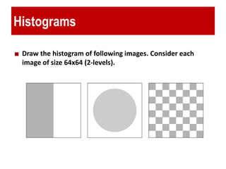
Histograms
A histogram for a grayscale image with intensity values in
range I(x, y) [0, L—1] would contain exactly L entries
E.g. 8-bit grayscale image, L = 2^8 = 256
Each histogram entry is defined as:
h(i) = number of pixels with intensity i for all 0 <= i< L.
E.g: h(255) = number of pixels with intensity = 255

Image Contrast
The contrast of a grayscale image indicates how easily
objects in the image can be distinguished
High contrast image: many distinct intensity values
Low contrast: image uses few intensity values

Uses for Histogram Processing
Image enhancements
Image statistics
Image compression
Image segmentation
Simple to calculate in software
Economic hardware implementations
Popular tool in real-time image processing
A plot of this function for all values of k provides a global
description of the appearance of the image (gives useful
information for contrast enhancement)

Uses for Histogram Processing
Four basic image types and their corresponding
histograms
– Dark
– Light
– Low contrast
– High contrast
Histograms commonly
viewed in plots as

2/16/2018 15

Dynamic Range
2/16/2018 16
• Dynamic Range: Number of distinct pixels in
image
• High dynamic range means very bright and very
dark parts in a single image (many distinct values)

2/16/2018 18
The intensity levels in an image may be viewed as
random variables in the interval [0, L-1].
Let ( ) and ( ) denote the probability density
function (PDF) of random variables and .
r sp r p s
r s

2/16/2018 19
( ) 0 1s T r r L   
. T(r) is a strictly monotonically increasing function
in the interval 0 -1;
. 0 ( ) -1 for 0 -1.
a
r L
b T r L r L
 
   

2/16/2018 20
. T(r) is a strictly monotonically increasing function
in the interval 0 -1;
. 0 ( ) -1 for 0 -1.
a
r L
b T r L r L
 
   
( ) 0 1s T r r L   
( ) is continuous and differentiable.T r
( ) ( )s rp s ds p r dr

0
( ) ( 1) ( )
r
rs T r L p w dw   
2/16/2018 21
0
( )
( 1) ( )
r
r
ds dT r d
L p w dw
dr dr dr
   
  
( 1) ( )rL p r 
 
( ) 1( ) ( )
( )
( 1) ( ) 1
r r r
s
r
p r dr p r p r
p s
L p rdsds L
dr
   
  
 
 

2/16/2018 22
Example
2
Suppose that the (continuous) intensity values
in an image have the PDF
2
, for 0 r L-1
( 1)( )
0, otherwise
Find the transformation function for equalizing
the image histogra
r
r
Lp r

 
 


m.

2/16/2018 23
Example
0
( ) ( 1) ( )
r
20
2
( 1)
( 1)
r w
L dw
L
 

2
1
r
L



2/16/2018 24
0
Continuous case:
( ) ( 1) ( )
r
0
Discrete values:
( ) ( 1) ( )
k
k k r j
j
s T r L p r

   
0 0
1
( 1) k=0,1,..., L-1
k k
j
j
j j
n L
L n
MN MN 

   

2/16/2018 25
Example: Histogram Equalization
Suppose that a 3-bit image (L=8) of size 64 × 64 pixels (MN = 4096) has the
intensity distribution shown in following table.
Get the histogram equalization transformation function and give the ps(sk)
for each sk.

2/16/2018 26
0
0 0
0
( ) 7 ( ) 7 0.19 1.33r j
j
s T r p r

     1
1
1 1
0
( ) 7 ( ) 7 (0.19 0.25) 3.08r j
j
s T r p r

      3
2 3
4 5
6 7
4.55 5 5.67 6
6.23 6 6.65 7
6.86 7 7.00 7
s s
s s
s s
   
   
   

2/16/2018 27

2/16/2018 30
Question
Is histogram equalization always good?

2/16/2018 31
Histogram Matching
Histogram matching (histogram specification)
— generate a processed image that has a specified histogram
Let ( ) and ( ) denote the continous probability
density functions of the variables and . ( ) is the
specified probability density function.
Let be the random variable with the prob
r z
z
p r p z
r z p z
s
0
0
ability
( ) ( 1) ( )
Define a random variable with the probability
( ) ( 1) ( )
r
r
z
z
s T r L p w dw
z
G z L p t dt s
  
  



2/16/2018 32
Histogram Matching
0
0
( ) ( 1) ( )
( ) ( 1) ( )
r
r
z
z
s T r L p w dw
G z L p t dt s
  
  


 1 1
( ) ( )z G s G T r 
 

2/16/2018 33
Histogram Matching: Procedure
• Obtain pr(r) from the input image and then obtain the values of s
• Use the specified PDF and obtain the transformation function G(z)
• Mapping from s to z
0
( 1) ( )
r
rs L p w dw  
0
( ) ( 1) ( )
z
zG z L p t dt s  
1
( )z G s


2/16/2018 34
Histogram Matching: Example
Assuming continuous intensity values, suppose that an image has the
intensity PDF
Find the transformation function that will produce an image whose
intensity PDF is
2
2
, for 0 -1
( 1)( )
0 , otherwise
r
r
r L
Lp r

 
 


2
3
3
, for 0 ( -1)
( ) ( 1)
0, otherwise
z
z
z L
p z L

 
 



Histogram Matching: Example
Find the histogram equalization transformation for the input image
Find the histogram equalization transformation for the specified histogram
The transformation function
20 0
2
( ) ( 1) ( ) ( 1)
( 1)
r r
r
w
s T r L p w dw L dw
L
    
 
2/16/2018 35
2 3
3 20 0
3
( ) ( 1) ( ) ( 1)
( 1) ( 1)
z z
z
t z
G z L p t dt L dt s
L L
     
  
2
1
r
L


1/32
1/3 1/32 2 2
( 1) ( 1) ( 1)
1
r
z L s L L r
L
 
             

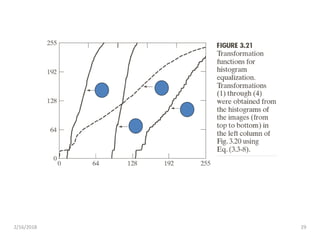
2/16/2018 36
Histogram Matching: Discrete Cases
• Obtain pr(rj) from the input image and then obtain the values of sk,
round the value to the integer range [0, L-1].
• Use the specified PDF and obtain the transformation function G(zq),
round the value to the integer range [0, L-1].
• Mapping from sk to zq
0 0
( 1)
( ) ( 1) ( )
k k
k k r j j
j j
L
s T r L p r n
MN 

    
0
( ) ( 1) ( )
q
q z i k
i
G z L p z s

  
1
( )q kz G s


2/16/2018 37
Example: Histogram Matching
Suppose that a 3-bit image (L=8) of size 64 × 64 pixels (MN = 4096) has the
intensity distribution shown in the following table (on the left). Get the
histogram transformation function and make the output image with the
specified histogram, listed in the table on the right.

2/16/2018
Obtain the scaled histogram-equalized values,
Compute all the values of the transformation function G,
0 1 2 3 4
5 6 7
1, 3, 5, 6, 7,
7, 7, 7.
s s s s s
s s s
    
  
0
0
0
( ) 7 ( ) 0.00z j
j
G z p z

 
1 2
3 4
5 6
7
( ) 0.00 ( ) 0.00
( ) 1.05 ( ) 2.45
( ) 4.55 ( ) 5.95
( ) 7.00
G z G z
G z G z
G z G z
G z
 
 
 

0
0 0
1 2
65
7

2/16/2018 39

2/16/2018 40
Obtain the scaled histogram-equalized values,
Compute all the values of the transformation function G,
0 1 2 3 4
5 6 7
1, 3, 5, 6, 7,
7, 7, 7.
s s s s s
s s s
    
  
0
0
0
( ) 7 ( ) 0.00z j
j
G z p z

 
1 2
3 4
5 6
7
( ) 0.00 ( ) 0.00
( ) 1.05 ( ) 2.45
( ) 4.55 ( ) 5.95
( ) 7.00
G z G z
G z G z
G z G z
G z
 
 
 

0
0 0
1 2
65
7
s0
s2 s3
s5 s6 s7
s1
s4

2/16/2018 41
0 1 2 3 4
5 6 7
1, 3, 5, 6, 7,
7, 7, 7.
s s s s s
s s s
    
  
0
1
2
3
4
5
6
7
kr

2/16/2018 42
0 3
1 4
2 5
3 6
4 7
5 7
6 7
7 7
k qr z









2/16/2018 43

2/16/2018 44

2/16/2018 45

2/16/2018 46
Local Histogram Processing
Define a neighborhood and move its center from pixel to pixel
At each location, the histogram of the points in the neighborhood
is computed. Either histogram equalization or histogram
specification transformation function is obtained
Map the intensity of the pixel centered in the neighborhood
Move to the next location and repeat the procedure

2/16/2018 47
Local Histogram Processing
• The two histogram processing methods discussed:
• Global
• pixels are modified by a transformation
function based on the gray-level content of an
entire image.
• Global approach is suitable for overall enhancement
• there are cases in which it is necessary to
enhance details over small areas in an image

2/16/2018 48
Local Histogram Processing: Example

2/16/2018 49
Using Histogram Statistics for Image
Enhancement
1
0
( )
L
i i
i
m r p r


 
1
0
( ) ( ) ( )
L
n
n i i
i
u r r m p r


 
1
2 2
2
0
( ) ( ) ( )
L
i i
i
u r r m p r


  
1 1
0 0
1
( , )
M N
x y
f x y
MN
 
 
 
 
1 1
2
0 0
1
( , )
M N
x y
f x y m
MN
 
 
 
Average Intensity
Variance

2/16/2018 50
Enhancement
1
0
Local average intensity
( )
denotes a neighborhood
xy xy
L
s i s i
i
xy
m r p r
s


 
1
2 2
0
Local variance
( ) ( )xy xy xy
L
s i s s i
i
r m p r


 

2/16/2018 51
Enhancement: Example
0 1 2
0 1 2
( , ), if and
( , )
( , ), otherwise
:global mean; :global standard deviation
0.4; 0.02; 0.4; 4
xy xys G G s G
G G
E f x y m k m k k
g x y
f x y
m
k k k E
  

  
 

   
g

Enhancement Using Arithmetic/Logic
Operations
Arithmetic/logic operations involving images
are performed on a pixel-by-pixel basis
between two or more images (this excludes
the logic operation NOT, which is performed
on a single image).
The difference between two images f(x, y) and
h(x, y), expressed as
G(x,y)=f(x,y)-h(x,y)

Basics of Spatial Filtering
The subimage is called a filter, mask,
kernel, template, or window.
The values in a filter subimage are referred to
as coefficients , rather than pixels.
Smoothing spatial filters

Histogram Processing

More Related Content

What's hot

Similar to Histogram Processing

More from Amnaakhaan

Recently uploaded

Histogram Processing