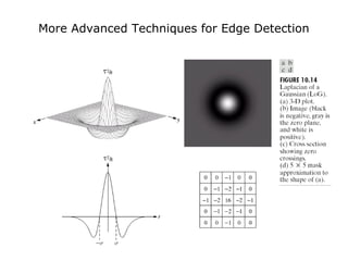
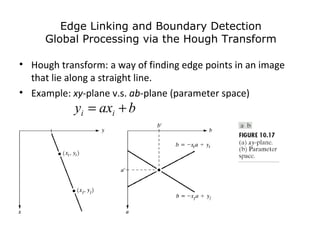
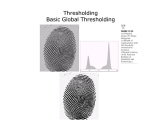
The document discusses various techniques for image segmentation including discontinuity-based approaches, similarity-based approaches, thresholding methods, region-based segmentation using region growing and region splitting/merging. Key techniques covered include edge detection using gradient operators, the Hough transform for edge linking, optimal thresholding, and split-and-merge segmentation using quadtrees.


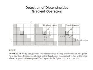
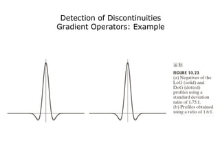
![Detection of Discontinuities
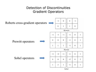
Gradient Operators
• First-order derivatives:
– The gradient of an image f(x,y) at location (x,y) is
defined as the vector:
– The magnitude of this vector:
– The direction of this vector:
– It points in the direction of the greatest rate of change
of f at location (x,y)
=
=∇
∂
∂
∂
∂
y
f
x
f
y
x
G
G
f
[ ] 2
1
22
)(mag yx GGf +=∇=∇ f
= −
y
x
G
G
yx 1
tan),(α](https://image.slidesharecdn.com/chapter10imagesegmentation-170804060314/85/Chapter10-image-segmentation-12-320.jpg)