![BACKGROUND
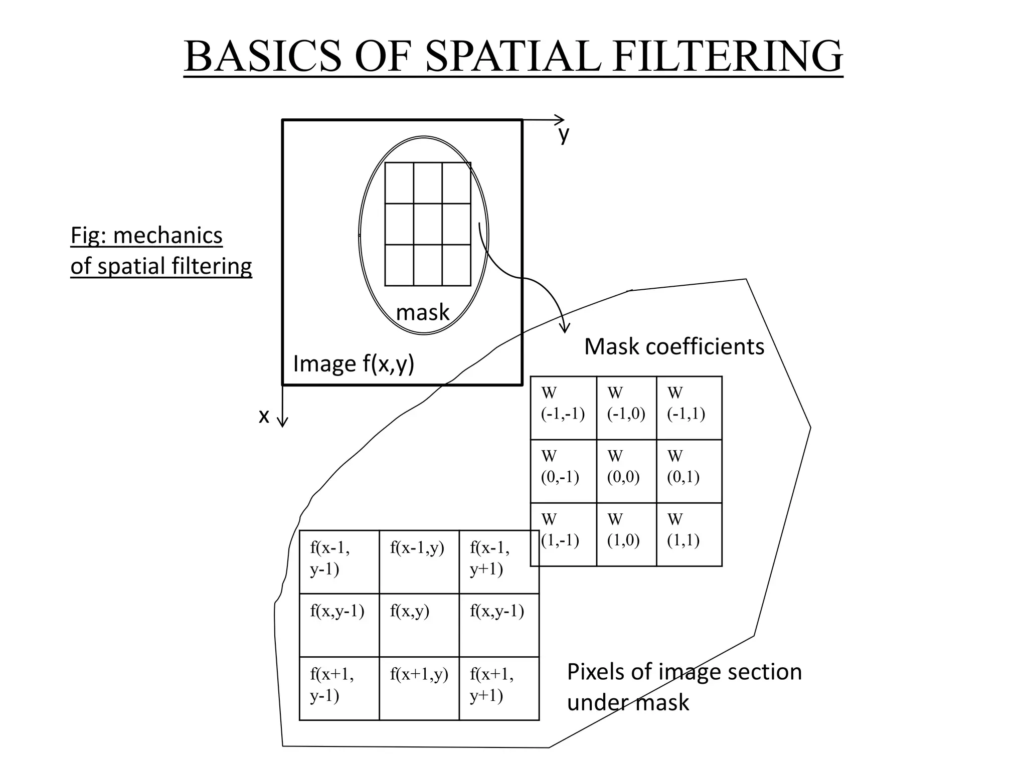
• Spatial domain processes are denoted by the expression
g(x,y) = T[f(x,y)]
where, f(x,y) is input image and g(x,y) is processed image,
T is an operator on f, defined over some neighborhood of (x,y)
• Square or Rectangular subimage area centered
at (x,y) is used as neighborhood
about a point (x,y).
• Here,
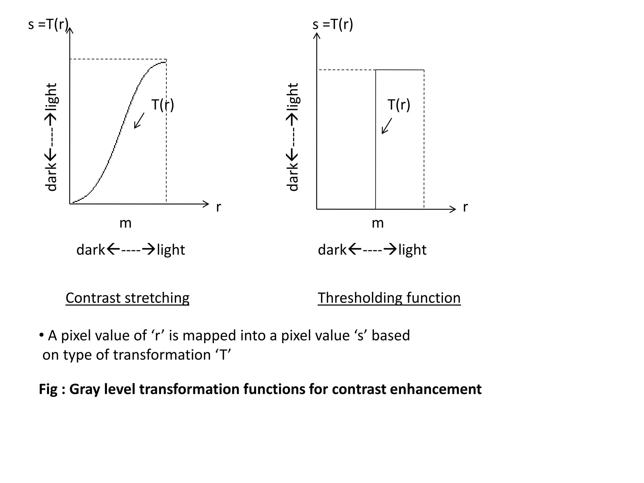
T is a gray level transformation function of the
form : s = T(r)
where, r and s – denote the gray levels of f(x,y)
and g(x,y) at any point (x,y). (x,y)
y
x
origin
Fig: 3 x 3 neighborhood about a point (x,y) in an image](https://image.slidesharecdn.com/imageenhancementinspatialdomain-140313122207-phpapp02/75/Image-Enhancement-in-Spatial-Domain-4-2048.jpg)
![BASIC GRAY LEVEL TRANSFORMATIONS
1. IMAGE NEGATIVES
• The negative of an image with gray
levels in the range[0,L-1] is obtained
using negative transformations as in fig.
and the expression is :
s = L-1- r
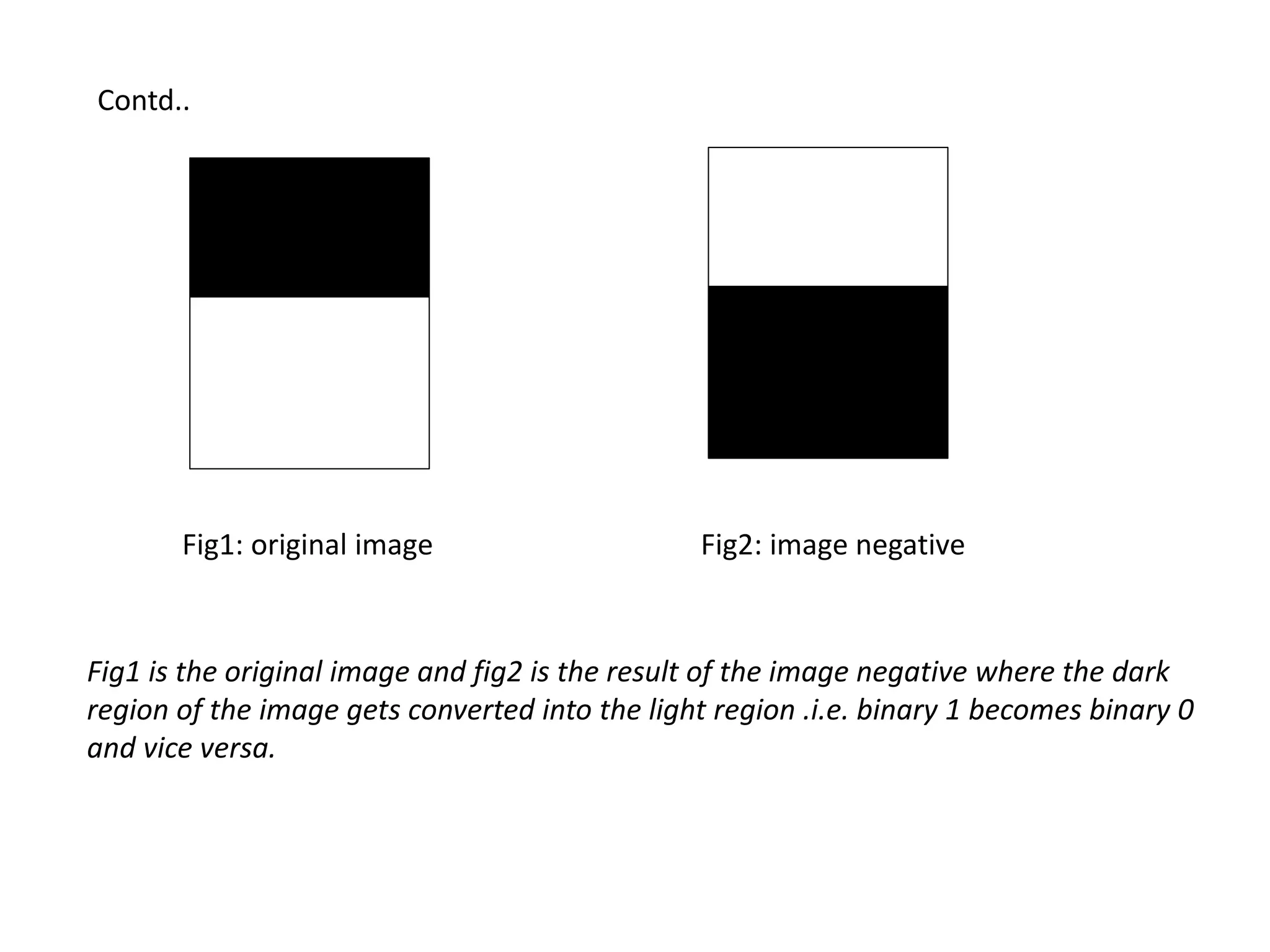
• This type of processing is particularly suited
for enhancing white or gray detail embedded
in dark regions of an image, especially
when the black area is dominant in size.
0 L-1
L-1
L/2
L/2](https://image.slidesharecdn.com/imageenhancementinspatialdomain-140313122207-phpapp02/75/Image-Enhancement-in-Spatial-Domain-6-2048.jpg)
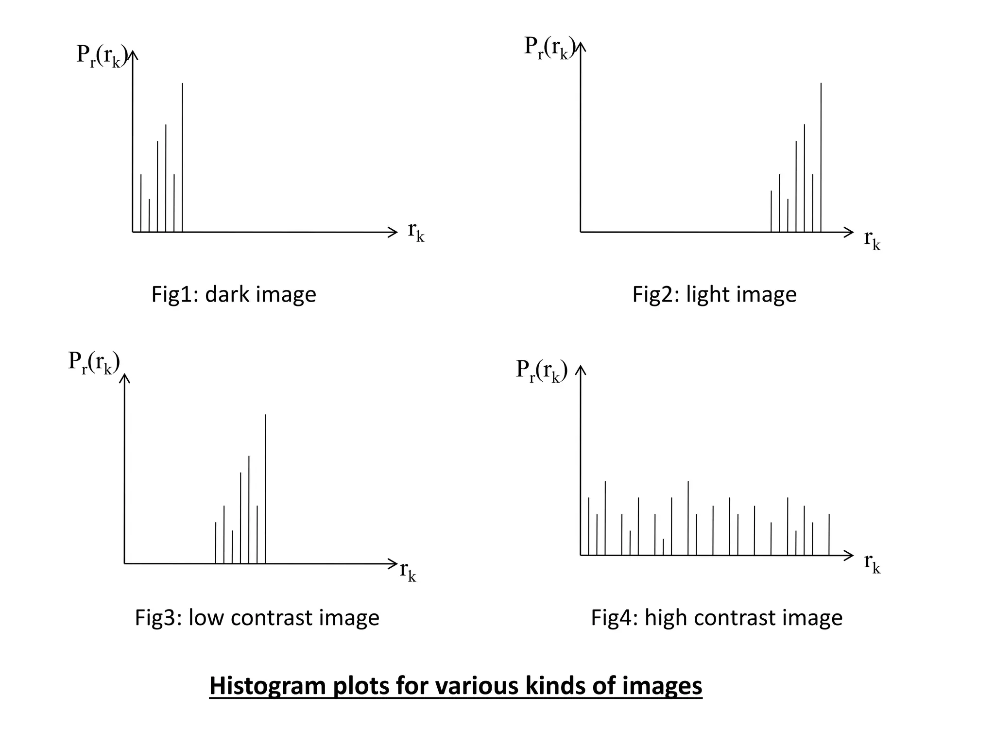
![HISTOGRAM PROCESSING
• The histogram of a digital image with gray levels in the range[0,L-1]
is a discrete function,
where, rk is the kth gray level & nk is number of pixels in the image
having gray level rk
• Histogram is normalized by dividing each of its values by the total
no. of pixels in the image denoted by ‘n’.
Thus normalized histogram is given by,
where, k = 0,1,2,….L-1
• Histograms are the basis for the numerous spatial domain processing
techniques.
• Histogram manipulation is used effectively for image enhancement,
also quite useful in other image processing applications viz image
compression & segmentation.](https://image.slidesharecdn.com/imageenhancementinspatialdomain-140313122207-phpapp02/75/Image-Enhancement-in-Spatial-Domain-14-2048.jpg)
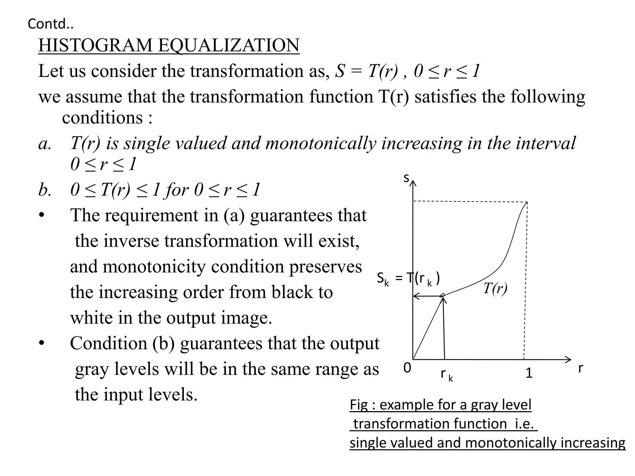
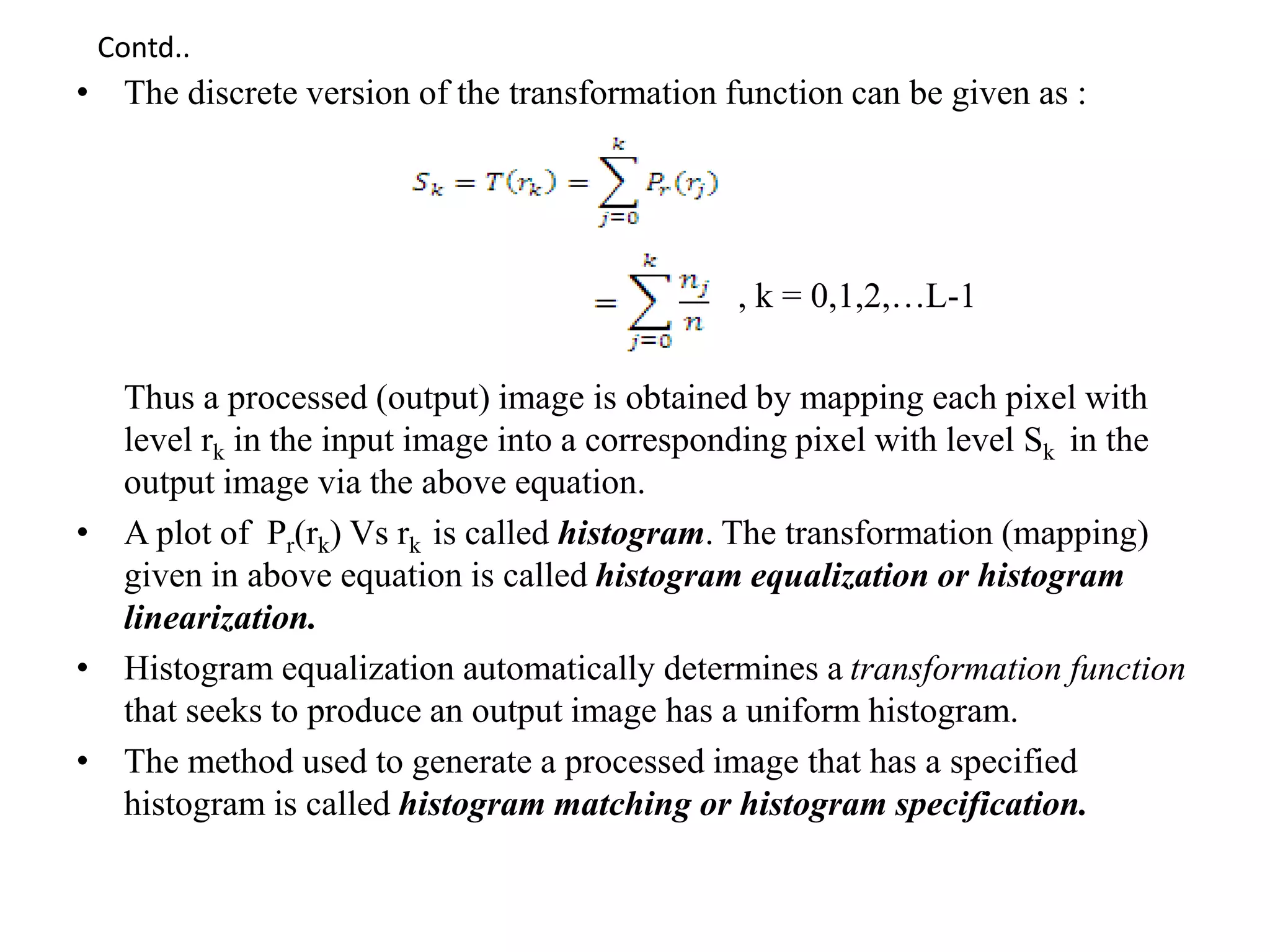

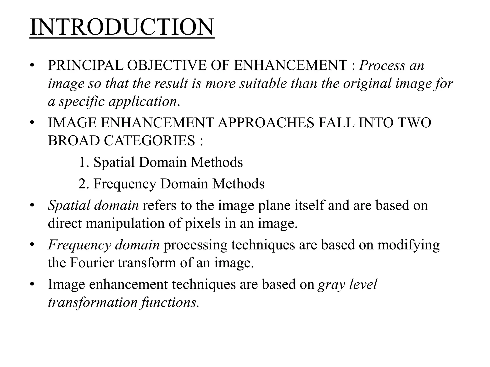
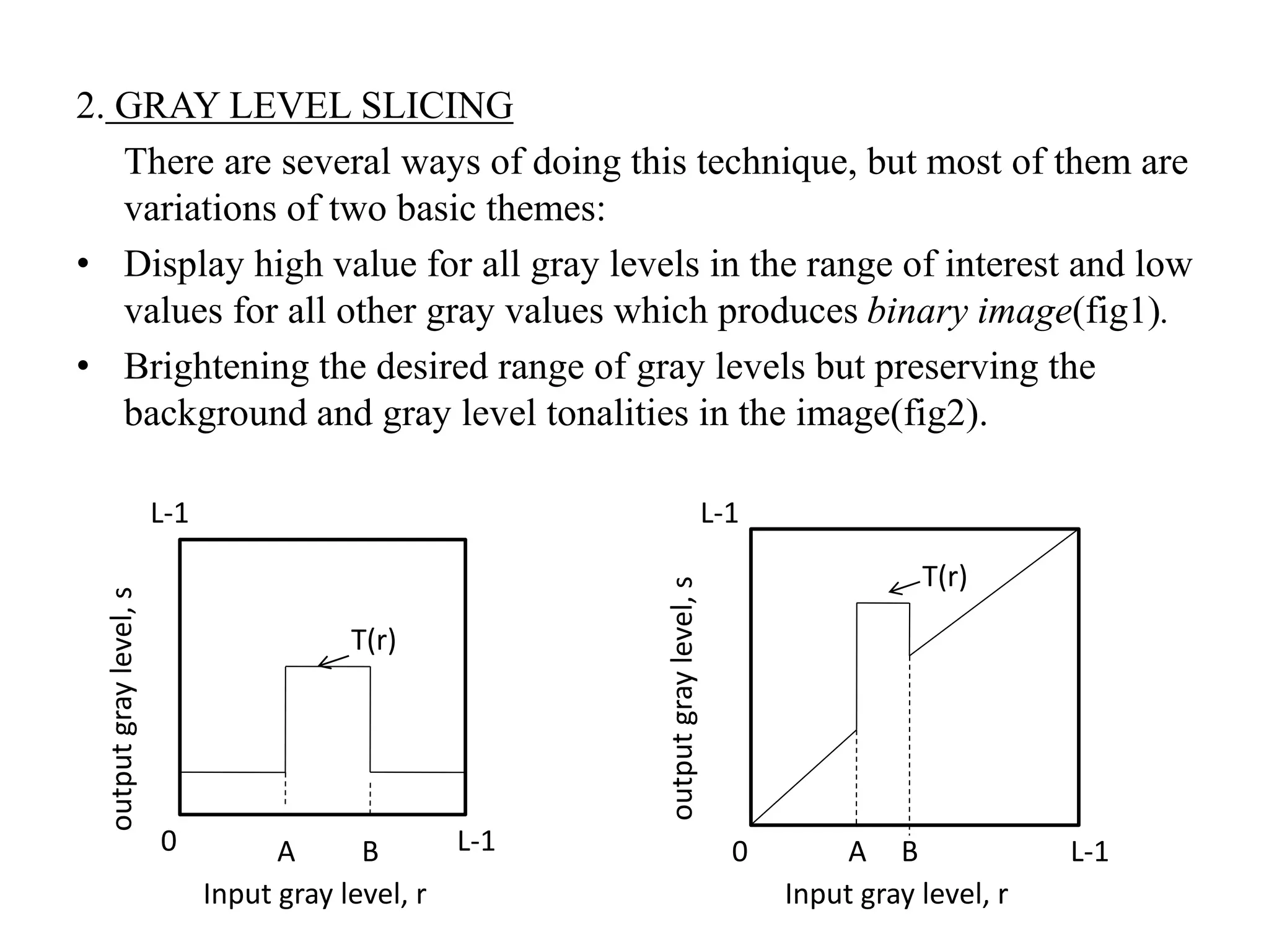
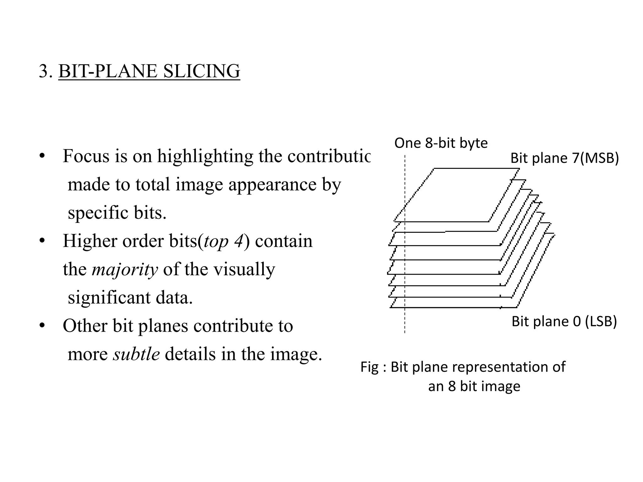
The document discusses various image enhancement techniques, focusing on gray level transformations, histogram processing, and spatial filtering methods. It categorizes enhancement approaches into spatial and frequency domain methods, detailing operations like image negatives, log transformations, and histogram equalization. Additionally, the document outlines the processes of local enhancement and image averaging, emphasizing the importance of manipulating pixel values for better visual representation in specific applications.