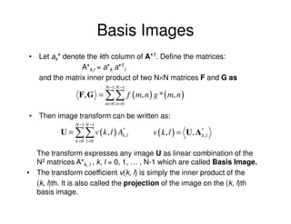
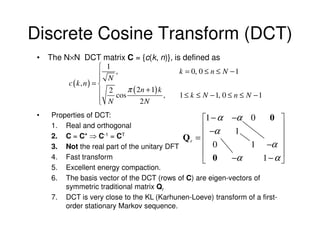
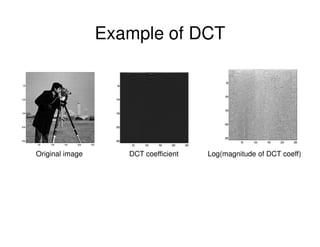
The document discusses various 2-D orthogonal and unitary transforms that can be used to represent digital images, including: 1. The discrete Fourier transform (DFT) which transforms an image into the frequency domain and has properties like energy conservation and fast computation via FFT. 2. The discrete cosine transform (DCT) which has good energy compaction properties and is close to the optimal Karhunen-Loeve transform. 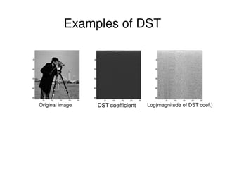3. The discrete sine transform (DST) which is real, symmetric, and orthogonal like the DCT. 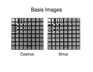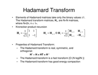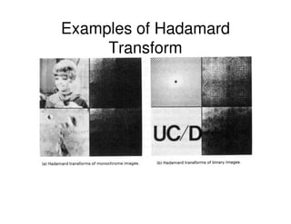4. The Hadamard transform which uses only ±1 values and has a fast computation, and the Haar transform which is a simpler wavelet transform

1. 03. Image Transforms
Tati R. Mengko

2. 2-D Orthogonal and Unitary Transforms
• Image transforms → refers to a class of unitary matrices which serves
as a basis for representing digital images.
– Unitary matrices : fullfills AA*T = ATA* = I
– Basis images : a discrete set of basis arrays that expands an image.
• For a N×N image, unitary transform of u(m, n) is given by:
N −1 N −1
u (m, n ) = ∑ ∑ v (k , l ) a * (m, n )
k =0 l =0
k ,l 0 ≤ m, n ≤ N − 1
N − 1 N −1
v (k , l ) = ∑ ∑ u (m, n ) a (m, n )
m =0 n=0
k ,l 0 ≤ k,l ≤ N −1
v(k, l) → transform coefficients
V ≡ {v(k, l)} → the transformed image
{ak,l (m, n)} → a set of complete orthonormal discrete basis functions
satisfying the properties: orthonormality and completeness.

3. 2-D Orthogonal and Unitary Transforms
N −1 N −1
ORTHONORMALITY: ∑∑ a ( m, n ) a * ( m, n ) = δ ( k − k ', l − l ')
m=0 n =0
k ,l k ',l '
N −1 N −1
COMPLETENESS : ∑∑ a ( m, n ) a * ( m ', n ') = δ ( m − m ', n − n ')
k =0 l =0
k ,l k ,l
• The orthonormality properties assures that any truncated series
expansion of the form:
P −1 Q −1
u P ,Q ( m, n ) ≡ ∑∑ v ( k , l ) a *k ,l ( m, n ) P ≤ N, Q ≤ N
k =0 l =0
N −1 N −1
σ = ∑∑ u ( m, n ) − u P ,Q ( m, n ) 
2 2
will minimize the sum of squared error e  
m =0 n =0
• The completeness property assures that this error will be zero for
P=Q=N.

4. Separable Unitary Transforms
• To reduce the computation order, transformation operation is desired
to be separable.
Separability:
ak ,l ( m, n ) = ak ( m ) al ( n ) ≡ a ( k , m ) b ( l , n )
{ak(m), k = 0, 1, …, N-1}
1-D complete orthogonal sets of basis vectors.
{bl(n), l = 0, 1, …, N-1}
→ Reduction of transformation computation order from O(N4) to O(N3) .
• Imposition of orthonormality and completeness on the unitary A ≡{a(k,
m)} and B ≡ {b(l, n)}, gives the following equation for B = A :
N −1 N −1
v ( k , l ) = ∑∑ a ( k , m ) u ( m, n ) a ( l , n ) ↔ V = AUAT
m =0 n =0
N −1 N −1
u ( m, n ) = ∑∑ a * ( k , m ) v ( k , l ) a * ( l , n ) ↔ U = A*T VA*
k =0 l =0

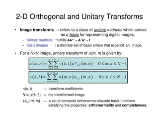
5. Separable Unitary Transforms
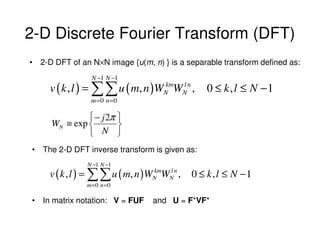
• For an M×N rectangular image, the transform pair is:
V = AMUAN and U = A*M V A*TN
• For separable unitary matrix, image transforms can be written as:
VT = AUAT = A [AU]T
Which means transformation process can be performed by first
transforming each column of U and then transforming each row of
the result to obtain the rows of V.

6. Basis Images
• Let ak* denote the kth column of A*T. Define the matrices:
A*k,l = a*k a*Tl
and the matrix inner product of two N×N matrices F and G as
N −1 N −1
F, G = ∑∑ f ( m, n ) g * ( m, n )
m =0 n =0
• Then image transform can be written as:
N −1 N −1
U = ∑∑ v ( k , l ) Ak ,l
*
v ( k , l ) = U , A * ,l
k
k =0 l =0
The transform expresses any image U as linear combination of the
N2 matrices A*k, l , k, l = 0, 1, … , N-1 which are called Basis Image.
• The transform coefficient v(k, l) is simply the inner product of the
(k, l)th. It is also called the projection of the image on the (k, l)th
basis image.

7. Basis Images
Cosinus Sinus

8. Basis Images
Hadamard Haar

9. Basis Images
Slant KLT

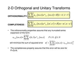
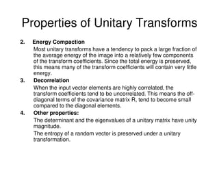
10. Properties of Unitary Transforms
1. Energy conservation and rotation
In a unitary transform:
v = Au ||v||2 = ||u||2
Thus a unitary transformation preserves the signal energy or the
length of the vector u in the N-dimensional vector space.
This means every unitary transformation is simply a rotation of the
vector u in the N-dimensional vector space. [Parseval Theorem!]
For 2-D unitary transformations, it can be proven that
N −1 N −1 N −1 N −1
∑∑ u ( m, n ) = ∑∑ v ( k , l )
2 2
m =0 n =0 k =0 l =0

11. Properties of Unitary Transforms
2. Energy Compaction
Most unitary transforms have a tendency to pack a large fraction of
the average energy of the image into a relatively few components
of the transform coefficients. Since the total energy is preserved,
this means many of the transform coefficients will contain very little
energy.
3. Decorrelation
When the input vector elements are highly correlated, the
transform coefficients tend to be uncorrelated. This means the off-
diagonal terms of the covariance matrix R, tend to become small
compared to the diagonal elements.
4. Other properties:
The determinant and the eigenvalues of a unitary matrix have unity
magnitude.
The entropy of a random vector is preserved under a unitary
transformation.

12. 2-D Discrete Fourier Transform (DFT)
• 2-D DFT of an N×N image {u(m, n) } is a separable transform defined as:
N −1 N −1
v ( k , l ) = ∑∑ u ( m, n )WN WN n ,
km l
0 ≤ k, l ≤ N −1
m =0 n =0
 − j 2π 
WN ≡ exp  
 N 
• The 2-D DFT inverse transform is given as:
N −1 N −1
v ( k , l ) = ∑∑ u ( m, n ) WN WN n ,
km l
0 ≤ k, l ≤ N −1
m=0 n =0
• In matrix notation: V = FUF and U = F*VF*

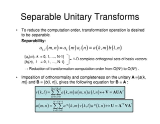
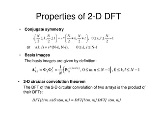
13. Properties of 2-D DFT
[The N2×N2 matrix F represents the N×N 2-D unitary DFT]
• Symmetric and unitary
F T = F and F –1 = F *
• Periodic extensions
v(k + N, l + N) = v(k, l) ∀k, l
u(m + N, n+N) = u(m, n) ∀m, n
• Sampled Fourier spectrum
If u ( m, n ) = u ( m, n ) , 0 ≤ m, n ≤ N − 1 ,and u ( m, n ) = 0 otherwise,
then:
%  2π k , 2π l  = DFT {u ( m, n )} = v ( k , lx )
U 
 N N 
where %
U (ω1 ,ω 2 ) is the Fourier transform of u ( m, n )
• Fast transform
Since 2-D DFT is separable, it is equivalent to 2N 1-D unitary DFTs, each of
which can be performed in O(N log2N) via the FFT. Hence the total number of
operations is O(N2 log2N).

14. Properties of 2-D DFT
• Conjugate symmetry
N N  N N  N
v  ± k, ± l  = v *  m k, m l , 0 ≤ k,l ≤ − 1
2 2  2 2  2
or v(k, l) = v*(N-k, N-l), 0 ≤ k, l ≤ N-1
• Basis Images
The basis images are given by definition:
1
A* , l = Φ k Φ T =
k l
N
{
WN (
− km + ln )
}
, 0 ≤ m, n ≤ N − 1 , 0 ≤ k , l ≤ N − 1
• 2-D circular convolution theorem
The DFT of the 2-D circular convolution of two arrays is the product of
their DFTs:
DFT{h(m, n)⊗ u(m, n)} = DFT{h(m, n)}.DFT{ u(m, n)}

15. Examples of DFT
50 50 50
100 100 100
150 150 150
200 200
200
250 250
250
50 100 150 200 250 50 100 150 200 250
50 100 150 200 250
Original Image Log(magnitude of DFT coeff) Phase Image

16. Discrete Cosine Transform (DCT)
• The N×N DCT matrix C = {c(k, n)}, is defined as
 1
 N, k = 0, 0 ≤ n ≤ N − 1

c (k, n) = 
 2 cos π ( 2n + 1) k , 1 ≤ k ≤ N − 1, 0 ≤ n ≤ N − 1
 N
 2N
• Properties of DCT:
1 − α −α 0 0 
1. Real and orthogonal  −α 1 
2. C = C* ⇒ C-1 = CT Qr =  
3. Not the real part of the unitary DFT  0 1 −α 
 
4. Fast transform  0 −α 1−α 
5. Excellent energy compaction.
6. The basis vector of the DCT (rows of C) are eigen-vectors of
symmetric traditional matrix Qr
7. DCT is very close to the KL (Karhunen-Loeve) transform of a first-
order stationary Markov sequence.

17. Example of DCT
50
50 50
100
100 100
150
150 150
200
200 200
250
250 250 50 100 150 200 250
50 100 150 200 250 50 100 150 200 250
Original image DCT coefficient Log(magnitude of DCT coeff)

18. Discrete Sine Transform (DST)
• The N×N DST matrix Ψ = {ψ(k, n)}, is defined as
2 π ( k + 1)( n + 1)
ψ ( k, n) = sin , 0 ≤ k, n ≤ N −1
N +1 N +1
• Properties of DST:
1. DST is real, symmetric, and orthogonal:
Ψ* = Ψ = ΨT = Ψ -1
2. DST is not the imaginary part of the unitary DFT
3. DST is a fast transform
4. The basis vectors of the DFT are the eigenvectors of the
symmetric tridiagonal Toeplitz matrix Q
5. DST is close to the KL transform of first order stationary
Markov sequences.
6. DST leads to a fast KL transform algorithm for Markov
sequence, whose boundary values are given.

19. Examples of DST
50 50 50
100 100 100
150 150 150
200 200 200
250 250 250
50 100 150 200 250 50 100 150 200 250 50 100 150 200 250
Original image DST coefficient Log(magnitude of DST coef.)

20. Hadamard Transform
• Elements of Hadamard matrices take only the binary values ±1.
The Hadamard transform matrices, Hn, are N×N matrices,
where N≡2n, n ∈ I+.
• Kronecker product recursion
1 1 1  1  H n −1 H n −1 
H1 = 1 −1 H n = H n −1 ⊗ H1 =  
2  2  H n −1 −H n −1 
• Properties of Hadamard Transform:
– The Hadamard transform is real, symmetric, and
orthogonal:
H* = H = HT = H-1
– The Hadamard transform is a fast transform {O (N log2N )}
– The Hadamard transform has good energy compaction

21. Examples of Hadamard
Transform

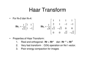
22. Haar Transform
• The Haar functions hk(x) are defined on a continuous interval,
x ∈[-1,1] and for k = 0, 1, …, N-1 where N=2n.
• The integer k can be uniquely decomposed as: k = 2p + q -1, where
0≤ p ≤n-1; q=0,1 for p=0 and 1≤ q ≤2p for p≠0.
• For Example, when N = 4 (or n=2) we have
k 0 1 2 3
p 0 0 1 1
q 0 1 1 2
Representing k by (p,q), the Haar functions are defined as:
1
h0 ( x ) ≡ h0,0 ( x ) = , x ∈ [ 0,1]
N
 p2 q −1 q −1 2
 2 , ≤x<
2p 2p

1  p 2 q −1 2 q
hk ( x ) ≡ hp ,q ( x ) =  −2 , ≤x< p
N  2p 2
0 , daerah lain untuk x ∈ [ 0,1]



23. Haar Transform
• For N=2 dan N=4:
 1 1 1 1 
 2 1 −1 −1 
1 1 1  1  
Hr2 = 1 −1 Hr8 =
2   4 2 − 2 0 0 
 

 0 0 2 − 2
• Properties of Haar Transform:
1. Real and orthogonal: Hr = Hr* dan Hr -1 = HrT
2. Very fast transform : O(N) operation on Nx1 vector.
3. Poor energy compaction for images

24. Slant Transform
• The N×N Slant transform matrices are defined by the recursion
 1 0 1 0  
a b 0 0 
 n n − an bn  S n −1 0  1 1 1 
1  0 I ( N / 2)−2 0 I ( N / 2)− 2    S1 = 1 −1
Sn =    2  
2 1 0 1 0  
 −b a 0 0 
bn an  0 S n −1 
 n n  
 0 I ( N / 2)−2 0 −I ( N / 2 ) − 2   
  
where N=2n and IM denotes an M×M identity matrix
• Parameters an dan bn are defined by the recursions:
bn = (1 + 4a2n-1)-1/2 a1 =1
 1 1 1 1 
an = 2bnan-1 
 3 1 −1 −3 

1 5 5 5 5
The 4×4 Slant transformation matrix: S 2 = 
1 
•
2 1 −1 −1

 1 −3 3 −1 
 
 5 5 5 5

25. Slant Transform Properties
• Properties:
1. Real and orthogonal: S = S* and S-1 = ST
2. A fast transform: O(N log2N)
3. Good energy compaction

26. KL Transform
• The KL transform was originally introduced as a series expansion for
continuous random processes by Karhunen and Louve.
• For a real N×1 random vector u, the basis vectors of the KL
transformation are given by the orthonormalized eigenvectors of its
autocorrelation matrix R:
Rφk = λk φk, 0≤ k ≤ N-1
• The KL transform of u is defined as: v = Φ*Tu
N −1
• And the inverse transform is: u = Φv = ∑ v ( k ) φk
k =0