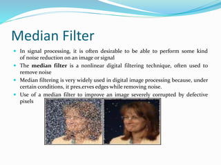
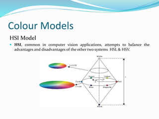
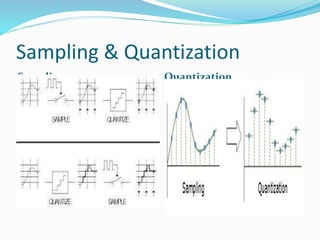
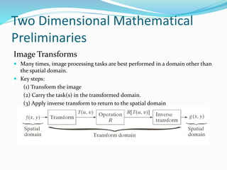
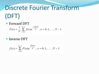
Digital Image Processing
IV-ECE(VII-SEM)
Submitted by
ABIRAMI M
AP/ECE
Introduction
 Digital image processing is the use of
computer algorithms to perform image
processing on digital images
 As a subcategory or field of digital signal processing,
digital image processing has many advantages
over analog image processing.
 Since images are defined over two dimensions
(perhaps more) digital image processing may be
modeled in the form of multidimensional systems
Fundamental Systems Image Processing Systems
Working Principles
VIDICON
The vidicon is a storage-type camera tube in which a charge-density pattern is
formed by the imaged scene radiation on a photoconductive surface which is then
scanned by a beam of low-velocity electrons. The fluctuating voltage coupled out
to a video amplifier can be used to reproduce the scene being imaged
Working Principles
Digital Camera
 Digital and film cameras share an optical system, typically using a lens with a
variable diaphragm to focus light onto an image pickup device.The diaphragm
and shutter admit the correct amount of light to the imager, just as with film
but the image pickup device is electronic rather than chemical.
 Most current consumer digital cameras use a Bayer filter mosaic in
combination with an optical anti-aliasing filter to reduce the aliasing due to the
reduced sampling of the different primary-color image
Working Principles
 Digital Camera
Elements of Visual Perception
Visual Perception
 Visual perception is the ability to interpret the surrounding environment by
processing information that is contained in visible light. The
resulting perception is also known as eyesight, sight, or vision
Mach Band Effect
 The Mach bands effect is due to the spatial high-boost filtering performed by
the human visual system on the luminance channel of the image captured by
the retina. This filtering is largely performed in the retina itself, by lateral
inhibition among its neurons.
Colour Models
RGB Model
 The RGB color model is an additive color model in which red, green,
and blue light are added together in various ways to reproduce a broad array
of colors.
 The main purpose of the RGB color model is for the sensing, representation,
and display of images in electronic systems, such as televisions and computers,
though it has also been used in conventional photography
Colour Models
 RGB Model
Colour Models
HSI Model
 HSI, common in computer vision applications, attempts to balance the
advantages and disadvantages of the other two systems HSL & HSV.
Sampling & Quantization
Sampling
 sampling is the reduction of a continuous signal to a discrete signal.
 A sample is a value or set of values at a point in time and/or space.
 A sampler is a subsystem or operation that extracts samples from a continuous
signal.
Quantization
 Quantization, involved in image processing, is a lossy compression technique
achieved by compressing a range of values to a single quantum value.
 When the number of discrete symbols in a given stream is reduced, the stream
becomes more compressible.
Sampling & Quantization
Sampling Quantization
Two Dimensional Mathematical
Preliminaries
Image Transforms
 Many times, image processing tasks are best performed in a domain other than
the spatial domain.
 Key steps:
(1) Transform the image
(2) Carry the task(s) in the transformed domain.
(3) Apply inverse transform to return to the spatial domain
Fourier Series Theorem
 Any periodic function f(t) can be expressed as a weighted sum (infinite) of sine
and cosine functions of varying frequency
is called the “fundamental frequency
Discrete Fourier Transform
(DFT)
Discrete Fourier Transform
(DFT)
 Forward DFT
 Inverse DFT
Discrete Cosine Transform A discrete cosine transform (DCT) expresses a finite sequence of data
points in terms of a sum of cosine functions oscillating at different frequencies.
 DCT is a Fourier-related transform similar to the discrete Fourier
transform (DFT), but using only real numbers. DCTs are equivalent to DFTs of
roughly twice the length, operating on real data with even symmetry. Types of
DCT listed below with 11 samples.
Karhunen–Loève Transform
(KLT)
 KLT is a representation of a stochastic process as an infinite linear
combination of orthogonal functions, analogous to a Fourier
series representation of a function on a bounded interval.
 In contrast to a Fourier series where the coefficients are fixed numbers and the
expansion basis consists of sinusoidal functions (that
is, sine and cosine functions), the coefficients in the Karhunen–Loève theorem
are random variables and the expansion basis depends on the process.
 Theorem. Let Xt be a zero-mean square integrable stochastic process defined
over a probability space (Ω, F, P) and indexed over a closed and bounded
interval [a, b], with continuous covariance function KX(s, t).
 Then KX(s,t) is a Mercer kernel and letting ek be an orthonormal basis
of L2([a, b]) formed by the eigenfunctions of TKX with respective eigenvalues λk,
Xt admits the following representation
 where the convergence is in L2, uniform in t and
Unit 2
Image Enhancement
Histogram Equalization
 This method usually increases the global contrast of many images, especially
when the usable data of the image is represented by close contrast values.
 This allows for areas of lower local contrast to gain a higher contrast. Histogram
equalization accomplishes this by effectively spreading out the most frequent
intensity values.
 Image before & after Histogram Equalization
Histogram equalization
• Basic idea: find a map f(x) such that the histogram of the
modified (equalized) image is flat (uniform).
• Key motivation: cumulative probability function (cdf) of
a random variable approximates a uniform distribution
• Suppose h(t) is the histogram


x
t
thxs
0
)()(
Histogram Equalization


x
t
thLy
0
)(
Uniform
Quantization


L
t
th
0
1)(Note:
L
1


x
t
ths
0
)(
x
L
y
0
cumulative probability function
Noise in Image Processing Noise means any unwanted signal
 One person’s signal is another one’s noise
 Noise is not always random and randomness is an artificial term
 Noise is not always bad
No Noise Light Noise Heavy Noise
Noise Removal Techniques
 Linear filtering
 Nonlinear filtering
Linear system
Spatial Averaging
 Here each pixel is replaced by a weighted average of its neighbourhood pixels
i.e.
 where and are i/pr opposite images. w is a suitably chosen window and are
the filter weights.
 A common class of spatial averaging filters has all equal weights giving
Directional Smoothing
 Smoothing is like a data set is to create an approximating function that
attempts to capture important patterns in the data, while leaving out noise or
other fine-scale structures/rapid phenomena.
Smoothing may be distinguished from the related and partially overlapping
concept of curve fitting in the following ways:
 curve fitting often involves the use of an explicit function form for the result,
whereas the immediate results from smoothing are the "smoothed" values with
no later use made of a functional form if there is one;
 the aim of smoothing is to give a general idea of relatively slow changes of value
with little attention paid to the close matching of data values, while curve
fitting concentrates on achieving as close a match as possible.
 smoothing methods often have an associated tuning parameter which is used
to control the extent of smoothing. Curve fitting will adjust any number of
parameters of the function to obtain the 'best' fit.
Median Filter
 In signal processing, it is often desirable to be able to perform some kind
of noise reduction on an image or signal
 The median filter is a nonlinear digital filtering technique, often used to
remove noise
 Median filtering is very widely used in digital image processing because, under
certain conditions, it pres.erves edges while removing noise.
 Use of a median filter to improve an image severely corrupted by defective
pixels
Types Of Filters
There are different kinds of mean filters all of which exhibit
slightly different behaviour:
• Geometric Mean
• Harmonic Mean
• Contraharmonic Mean
Geometric Mean
Geometric Mean:
Achieves similar smoothing to the arithmetic mean, but
tends to lose less image detail
mn
Sts xy
tsgyxf
1
),(
),(),(ˆ








 
Harmonic Mean
Harmonic Mean:
Works well for salt noise, but fails for pepper noise.
Also does well for other kinds of noise such as Gaussian
noise.


xySts tsg
mn
yxf
),( ),(
1
),(ˆ
Contraharmonic Mean
Contraharmonic Mean:
Q is the order of the filter.
Positive values of Q eliminate pepper noise.
Negative values of Q eliminate salt noise.
It cannot eliminate both simultaneously.






xy
xy
Sts
Q
Sts
Q
tsg
tsg
yxf
),(
),(
1
),(
),(
),(ˆ
Homomorphic filtering
 Homomorphic filtering is a generalized technique for signal and image
processing, involving a nonlinear mapping to a different domain in which
linear filter techniques are applied, followed by mapping back to the original
domain.
 Homomorphic filter is sometimes used for image enhancement. It
simultaneously normalizes the brightness across an image and increases
contrast.
 Here homomorphic filtering is used to remove multiplicative noise.
Illumination and reflectance are not separable, but their approximate locations
in the frequency domain may be located.
 Homomorphic filtering is used in the log-spectral domain to separate filter
effects from excitation effects, for example in the computation of
the cepstrum as a sound representation; enhancements in the log spectral
domain can improve sound intelligibility, for example in hearing aids

Digital image processing

  • 1.
  • 2.
    Introduction  Digital imageprocessing is the use of computer algorithms to perform image processing on digital images  As a subcategory or field of digital signal processing, digital image processing has many advantages over analog image processing.  Since images are defined over two dimensions (perhaps more) digital image processing may be modeled in the form of multidimensional systems
  • 3.
    Fundamental Systems ImageProcessing Systems
  • 4.
    Working Principles VIDICON The vidiconis a storage-type camera tube in which a charge-density pattern is formed by the imaged scene radiation on a photoconductive surface which is then scanned by a beam of low-velocity electrons. The fluctuating voltage coupled out to a video amplifier can be used to reproduce the scene being imaged
  • 5.
    Working Principles Digital Camera Digital and film cameras share an optical system, typically using a lens with a variable diaphragm to focus light onto an image pickup device.The diaphragm and shutter admit the correct amount of light to the imager, just as with film but the image pickup device is electronic rather than chemical.  Most current consumer digital cameras use a Bayer filter mosaic in combination with an optical anti-aliasing filter to reduce the aliasing due to the reduced sampling of the different primary-color image
  • 6.
  • 7.
    Elements of VisualPerception Visual Perception  Visual perception is the ability to interpret the surrounding environment by processing information that is contained in visible light. The resulting perception is also known as eyesight, sight, or vision
  • 8.
    Mach Band Effect The Mach bands effect is due to the spatial high-boost filtering performed by the human visual system on the luminance channel of the image captured by the retina. This filtering is largely performed in the retina itself, by lateral inhibition among its neurons.
  • 9.
    Colour Models RGB Model The RGB color model is an additive color model in which red, green, and blue light are added together in various ways to reproduce a broad array of colors.  The main purpose of the RGB color model is for the sensing, representation, and display of images in electronic systems, such as televisions and computers, though it has also been used in conventional photography
  • 10.
  • 11.
    Colour Models HSI Model HSI, common in computer vision applications, attempts to balance the advantages and disadvantages of the other two systems HSL & HSV.
  • 12.
    Sampling & Quantization Sampling sampling is the reduction of a continuous signal to a discrete signal.  A sample is a value or set of values at a point in time and/or space.  A sampler is a subsystem or operation that extracts samples from a continuous signal. Quantization  Quantization, involved in image processing, is a lossy compression technique achieved by compressing a range of values to a single quantum value.  When the number of discrete symbols in a given stream is reduced, the stream becomes more compressible.
  • 13.
  • 14.
    Two Dimensional Mathematical Preliminaries ImageTransforms  Many times, image processing tasks are best performed in a domain other than the spatial domain.  Key steps: (1) Transform the image (2) Carry the task(s) in the transformed domain. (3) Apply inverse transform to return to the spatial domain
  • 15.
    Fourier Series Theorem Any periodic function f(t) can be expressed as a weighted sum (infinite) of sine and cosine functions of varying frequency is called the “fundamental frequency
  • 16.
  • 17.
    Discrete Fourier Transform (DFT) Forward DFT  Inverse DFT
  • 18.
    Discrete Cosine TransformA discrete cosine transform (DCT) expresses a finite sequence of data points in terms of a sum of cosine functions oscillating at different frequencies.  DCT is a Fourier-related transform similar to the discrete Fourier transform (DFT), but using only real numbers. DCTs are equivalent to DFTs of roughly twice the length, operating on real data with even symmetry. Types of DCT listed below with 11 samples.
  • 19.
    Karhunen–Loève Transform (KLT)  KLTis a representation of a stochastic process as an infinite linear combination of orthogonal functions, analogous to a Fourier series representation of a function on a bounded interval.  In contrast to a Fourier series where the coefficients are fixed numbers and the expansion basis consists of sinusoidal functions (that is, sine and cosine functions), the coefficients in the Karhunen–Loève theorem are random variables and the expansion basis depends on the process.  Theorem. Let Xt be a zero-mean square integrable stochastic process defined over a probability space (Ω, F, P) and indexed over a closed and bounded interval [a, b], with continuous covariance function KX(s, t).  Then KX(s,t) is a Mercer kernel and letting ek be an orthonormal basis of L2([a, b]) formed by the eigenfunctions of TKX with respective eigenvalues λk, Xt admits the following representation  where the convergence is in L2, uniform in t and
  • 20.
  • 21.
    Image Enhancement Histogram Equalization This method usually increases the global contrast of many images, especially when the usable data of the image is represented by close contrast values.  This allows for areas of lower local contrast to gain a higher contrast. Histogram equalization accomplishes this by effectively spreading out the most frequent intensity values.  Image before & after Histogram Equalization
  • 22.
    Histogram equalization • Basicidea: find a map f(x) such that the histogram of the modified (equalized) image is flat (uniform). • Key motivation: cumulative probability function (cdf) of a random variable approximates a uniform distribution • Suppose h(t) is the histogram   x t thxs 0 )()(
  • 23.
  • 24.
    Noise in ImageProcessing Noise means any unwanted signal  One person’s signal is another one’s noise  Noise is not always random and randomness is an artificial term  Noise is not always bad No Noise Light Noise Heavy Noise
  • 25.
    Noise Removal Techniques Linear filtering  Nonlinear filtering Linear system
  • 26.
    Spatial Averaging  Hereeach pixel is replaced by a weighted average of its neighbourhood pixels i.e.  where and are i/pr opposite images. w is a suitably chosen window and are the filter weights.  A common class of spatial averaging filters has all equal weights giving
  • 27.
    Directional Smoothing  Smoothingis like a data set is to create an approximating function that attempts to capture important patterns in the data, while leaving out noise or other fine-scale structures/rapid phenomena. Smoothing may be distinguished from the related and partially overlapping concept of curve fitting in the following ways:  curve fitting often involves the use of an explicit function form for the result, whereas the immediate results from smoothing are the "smoothed" values with no later use made of a functional form if there is one;  the aim of smoothing is to give a general idea of relatively slow changes of value with little attention paid to the close matching of data values, while curve fitting concentrates on achieving as close a match as possible.  smoothing methods often have an associated tuning parameter which is used to control the extent of smoothing. Curve fitting will adjust any number of parameters of the function to obtain the 'best' fit.
  • 28.
    Median Filter  Insignal processing, it is often desirable to be able to perform some kind of noise reduction on an image or signal  The median filter is a nonlinear digital filtering technique, often used to remove noise  Median filtering is very widely used in digital image processing because, under certain conditions, it pres.erves edges while removing noise.  Use of a median filter to improve an image severely corrupted by defective pixels
  • 29.
    Types Of Filters Thereare different kinds of mean filters all of which exhibit slightly different behaviour: • Geometric Mean • Harmonic Mean • Contraharmonic Mean
  • 30.
    Geometric Mean Geometric Mean: Achievessimilar smoothing to the arithmetic mean, but tends to lose less image detail mn Sts xy tsgyxf 1 ),( ),(),(ˆ          
  • 31.
    Harmonic Mean Harmonic Mean: Workswell for salt noise, but fails for pepper noise. Also does well for other kinds of noise such as Gaussian noise.   xySts tsg mn yxf ),( ),( 1 ),(ˆ
  • 32.
    Contraharmonic Mean Contraharmonic Mean: Qis the order of the filter. Positive values of Q eliminate pepper noise. Negative values of Q eliminate salt noise. It cannot eliminate both simultaneously.       xy xy Sts Q Sts Q tsg tsg yxf ),( ),( 1 ),( ),( ),(ˆ
  • 33.
    Homomorphic filtering  Homomorphicfiltering is a generalized technique for signal and image processing, involving a nonlinear mapping to a different domain in which linear filter techniques are applied, followed by mapping back to the original domain.  Homomorphic filter is sometimes used for image enhancement. It simultaneously normalizes the brightness across an image and increases contrast.  Here homomorphic filtering is used to remove multiplicative noise. Illumination and reflectance are not separable, but their approximate locations in the frequency domain may be located.  Homomorphic filtering is used in the log-spectral domain to separate filter effects from excitation effects, for example in the computation of the cepstrum as a sound representation; enhancements in the log spectral domain can improve sound intelligibility, for example in hearing aids