Downloaded 281 times


This document provides an introduction to wavelet transforms and their applications in data analysis, signal processing, and image processing. It discusses how wavelet transforms overcome limitations of Fourier transforms by using localized basis functions. Applications mentioned include decomposing signals into different frequency components over time and removing noise from data. Examples are provided to illustrate wavelet decomposition and denoising.


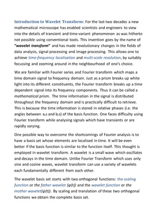
![Ch2 rev[1]](https://cdn.slidesharecdn.com/ss_thumbnails/ch2rev1-111122190305-phpapp01-thumbnail.jpg?width=640&height=640&fit=bounds)