Downloaded 44 times
![Fourier Transform - continued
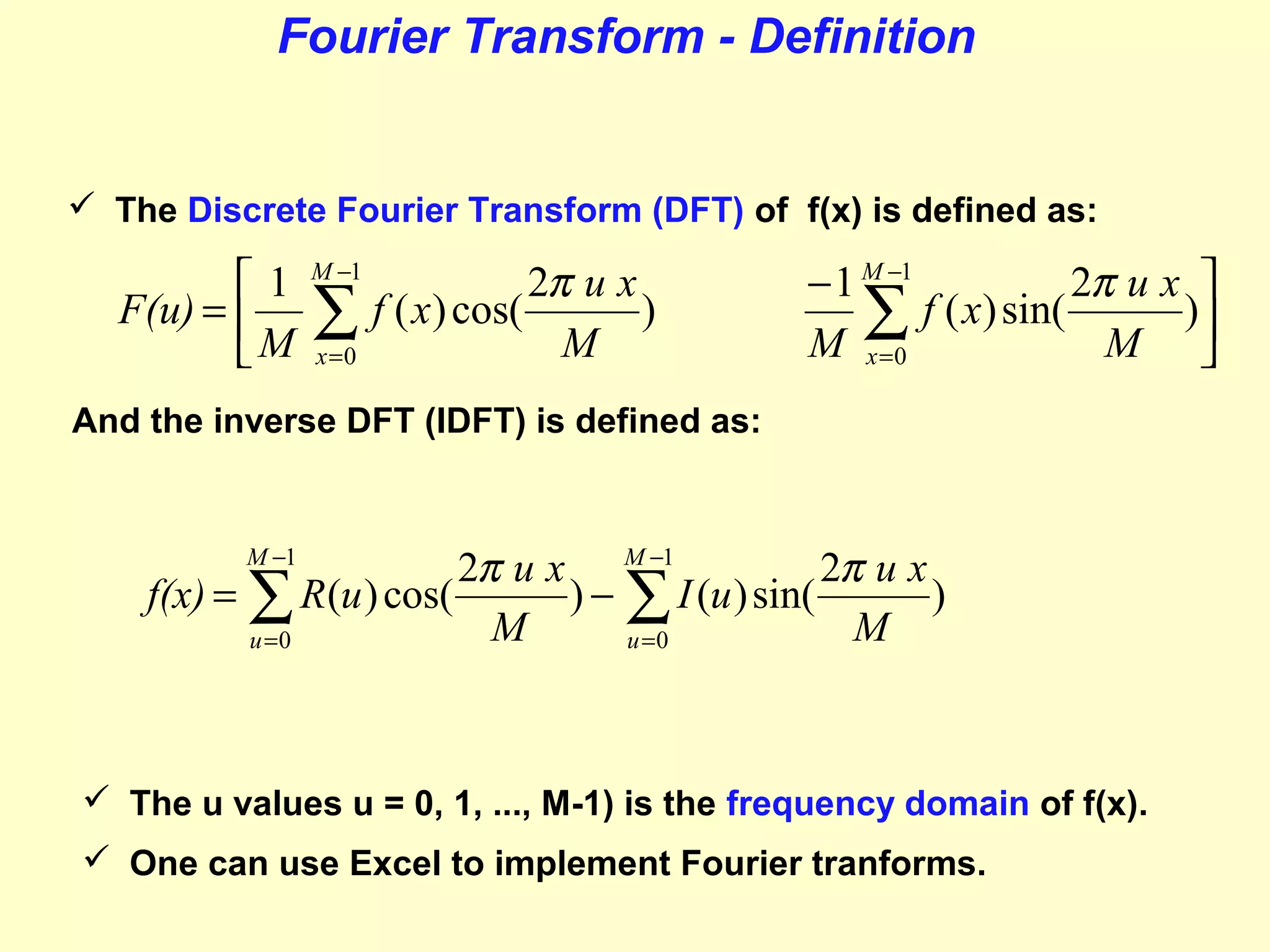
Unlike f(x), F(u) is a complex valued function, i.e. is a pair of
functions involving trigonometric functions:
1
R(u) =
M
I(u) = −
1
M
M −1
∑ f ( x) cos(2πux / M ),
called the real part, and
x =0
M −1
∑ f ( x) sin(2πux / M ),
called the imaginary part.
x =0
i.e. F(u) ≡ [ R(u ) I (u )].
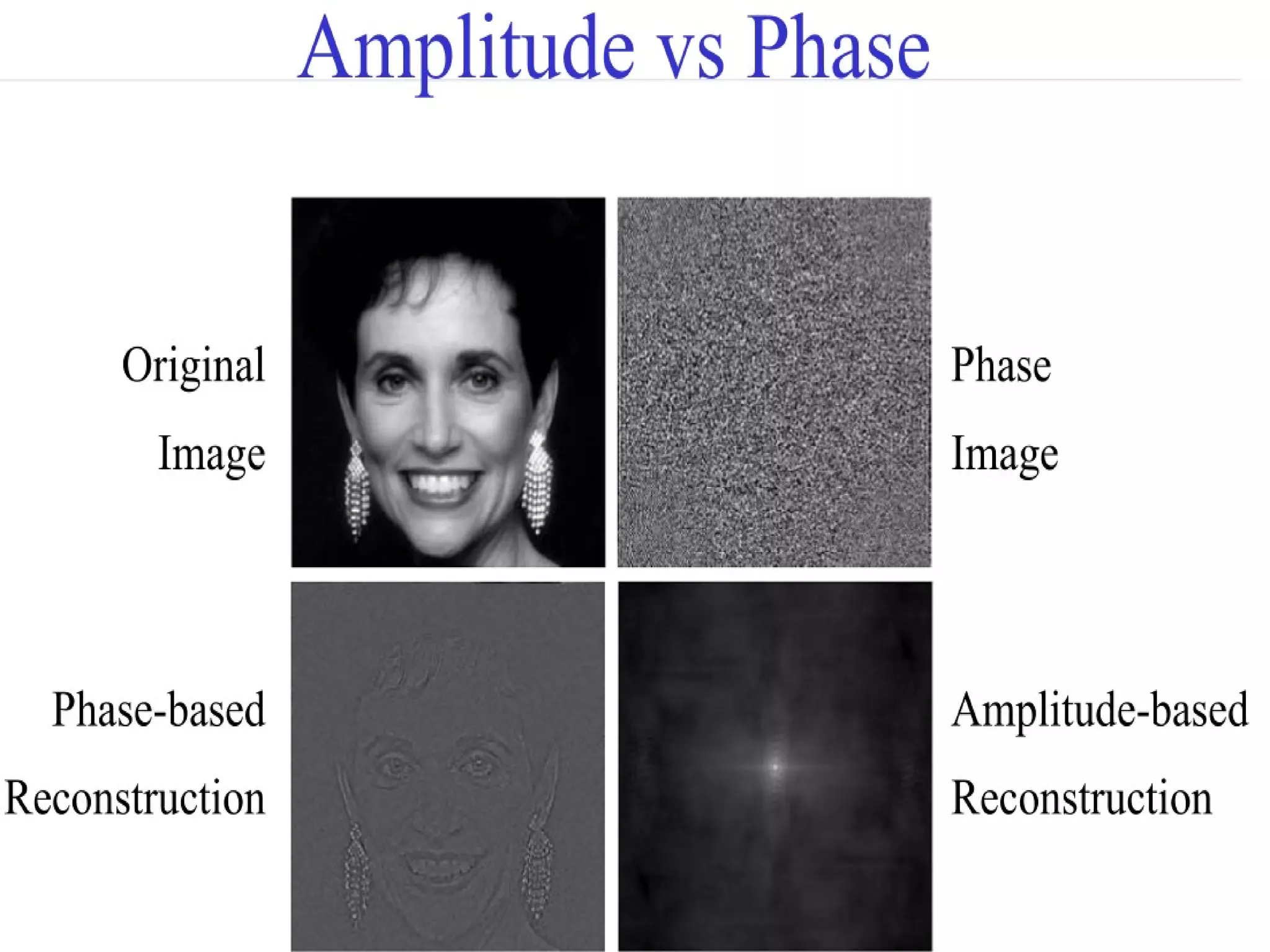
F is represented by its MAGNITUDE and PHASE rather that its
REAL and IMAGINARY parts,
where: MAGNITUDE(u) = SQRT( R(u)^2+IMAGINARY(u)^2 )
The phase angle of the transform is:
I (u )
φ (u ) = tan (
).
R(u )
−1
PHASE(u) = ATAN( IMAGINARY(u)/REAL(u) )](https://image.slidesharecdn.com/dip3-enhancementfreqdomain-131123025336-phpapp01/75/Digital-Image-Processing_-ch3-enhancement-freq-domain-9-2048.jpg)
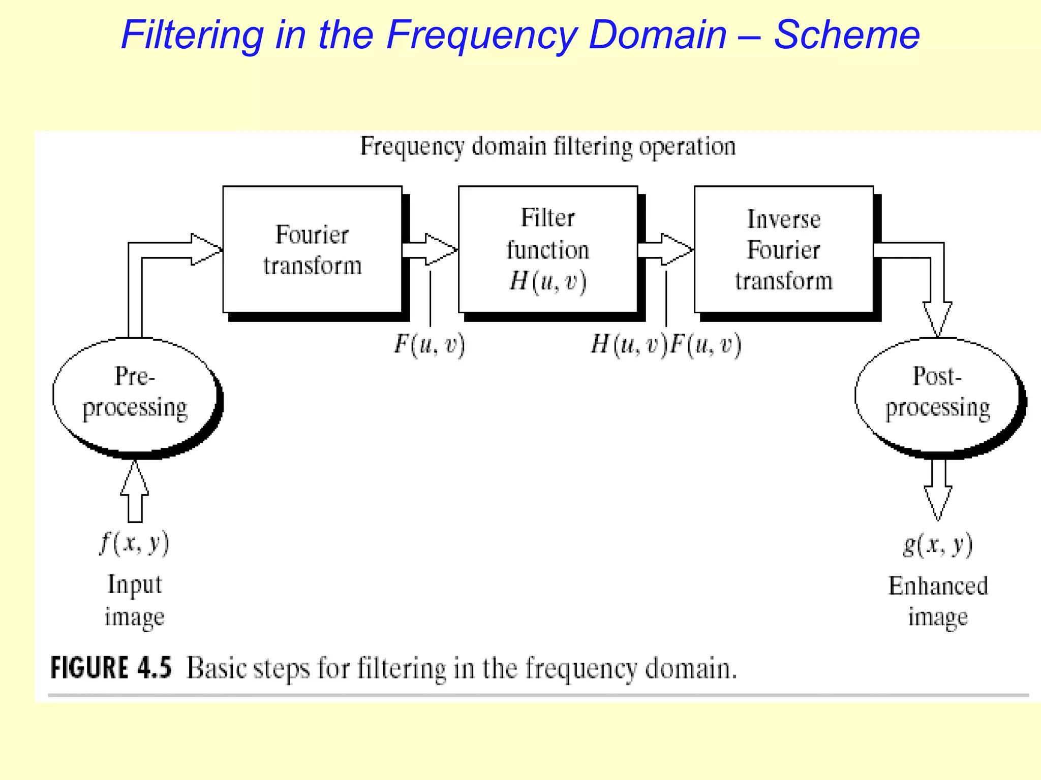
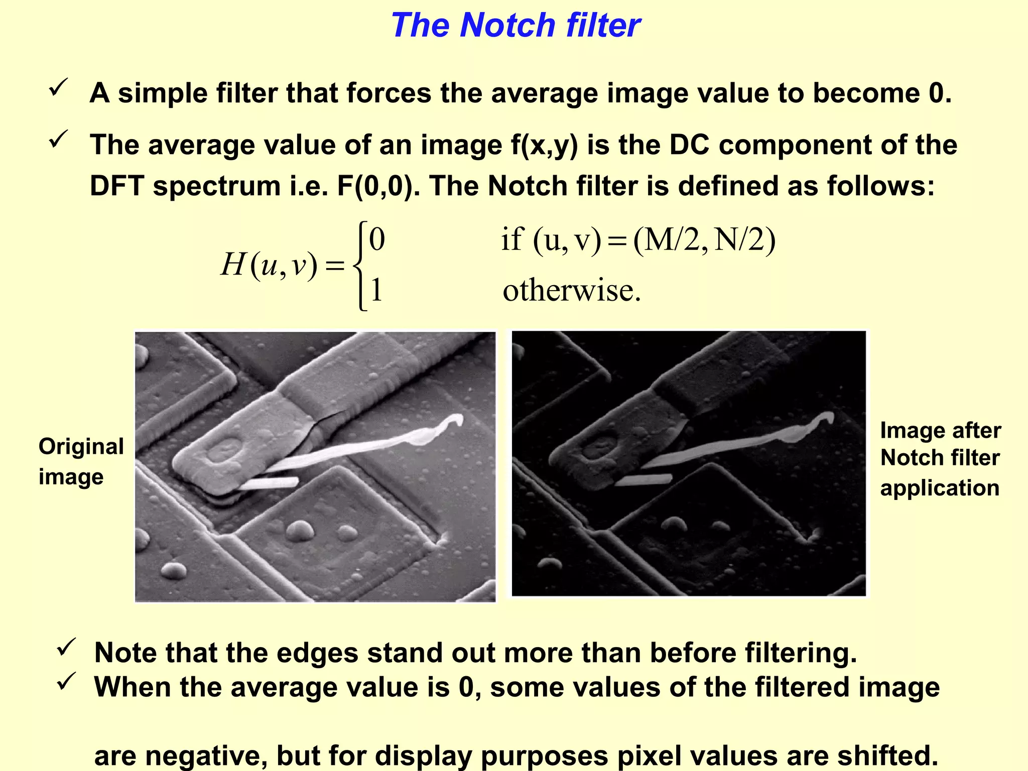
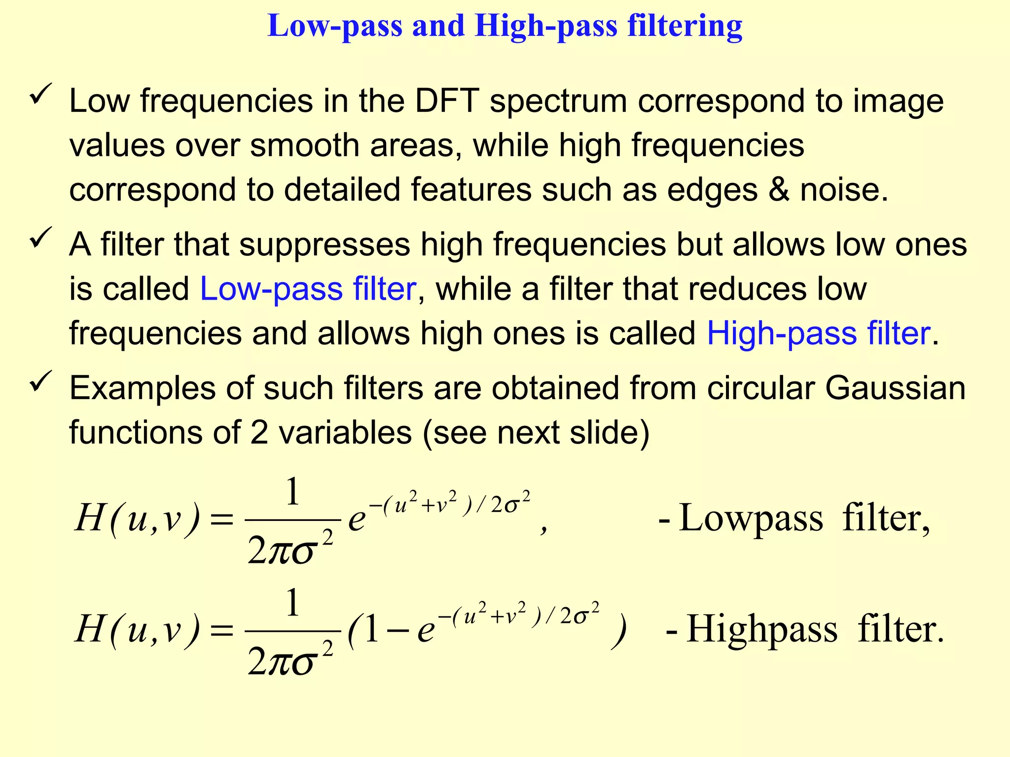
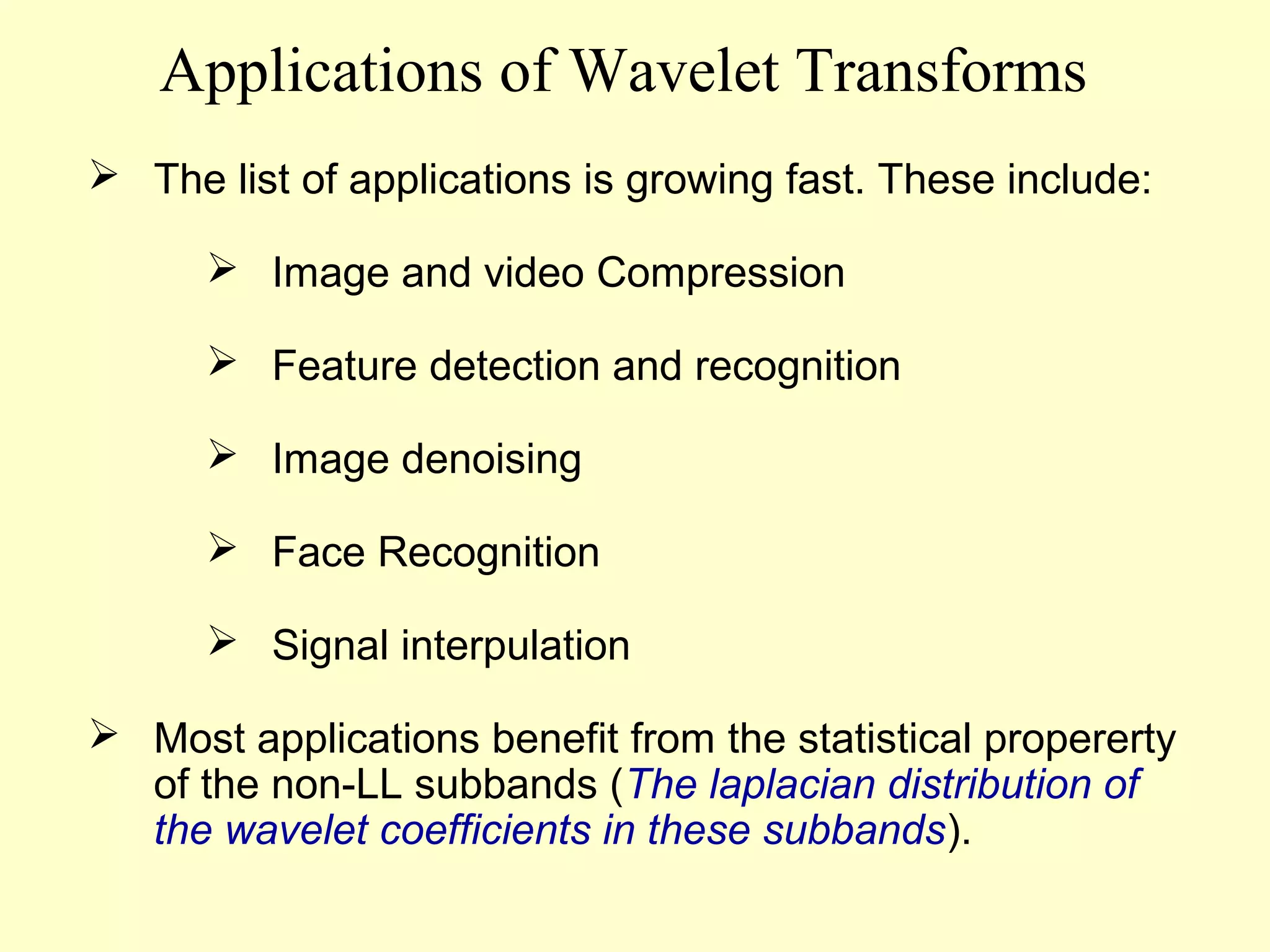
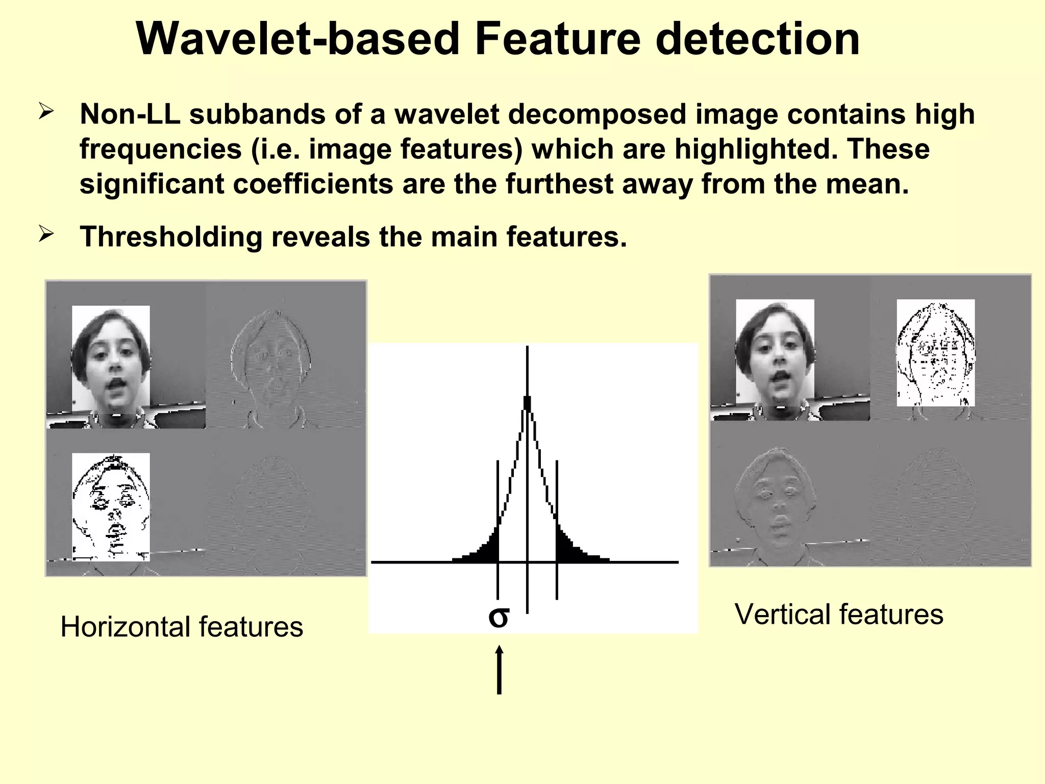
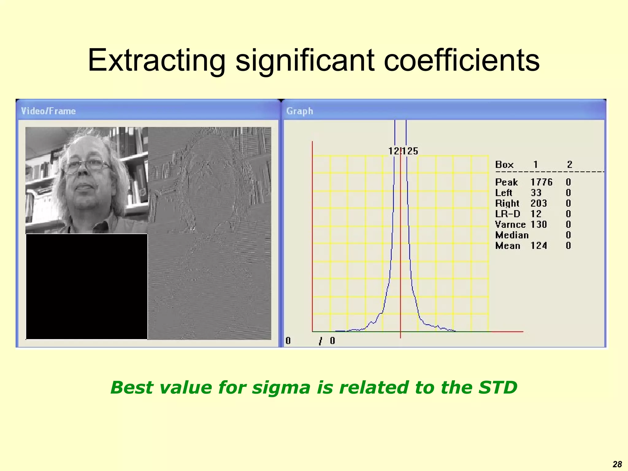
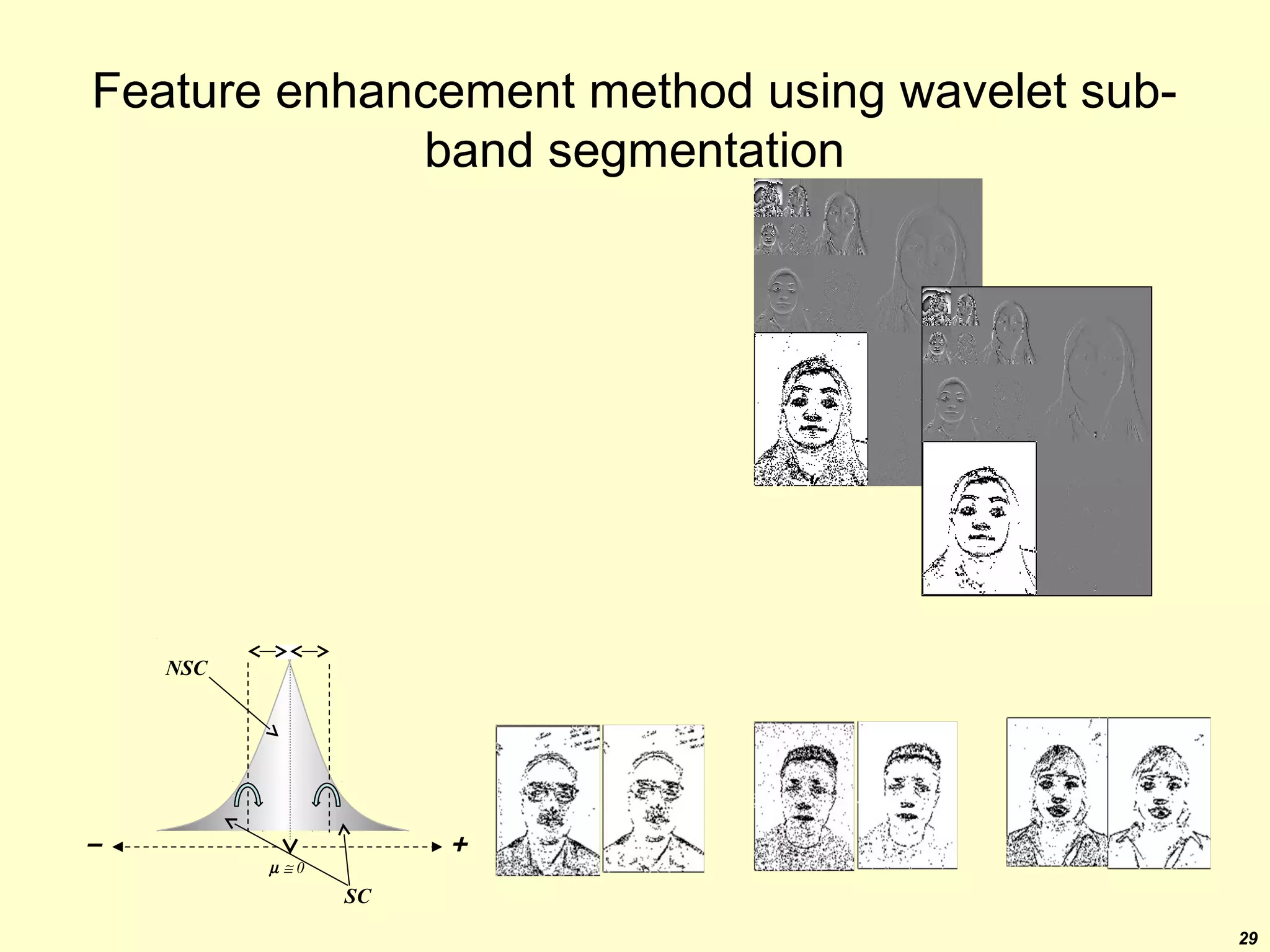


This chapter discusses frequency domain processing and image analysis using Fourier and wavelet transforms. It begins with an introduction to the frequency domain and Fourier transforms. The chapter then covers the definitions and properties of the discrete Fourier transform (DFT) and its application to images. Filtering techniques in the frequency domain like low-pass, high-pass and notch filters are described. The chapter also introduces wavelet transforms, including the discrete wavelet transform and Haar wavelets. Different wavelet decomposition schemes and the statistical properties of wavelet subbands are discussed. Finally, some applications of wavelet transforms like image compression, denoising and feature detection are mentioned.